We present considerations involved in finding the best location for the
compact (maximum antenna separation
![]() 200 m) ALMA configuration on
the science preserve. Several candidate locations for the compact
configuration are then suggested. Note that we distinguish here
between the compact ALMA configuration and the so-called ``Atacama
Compact Array'' (or ACA) which is a separate collection of smaller
antennas. We do not consider the placement of the ACA in this memo.
200 m) ALMA configuration on
the science preserve. Several candidate locations for the compact
configuration are then suggested. Note that we distinguish here
between the compact ALMA configuration and the so-called ``Atacama
Compact Array'' (or ACA) which is a separate collection of smaller
antennas. We do not consider the placement of the ACA in this memo.
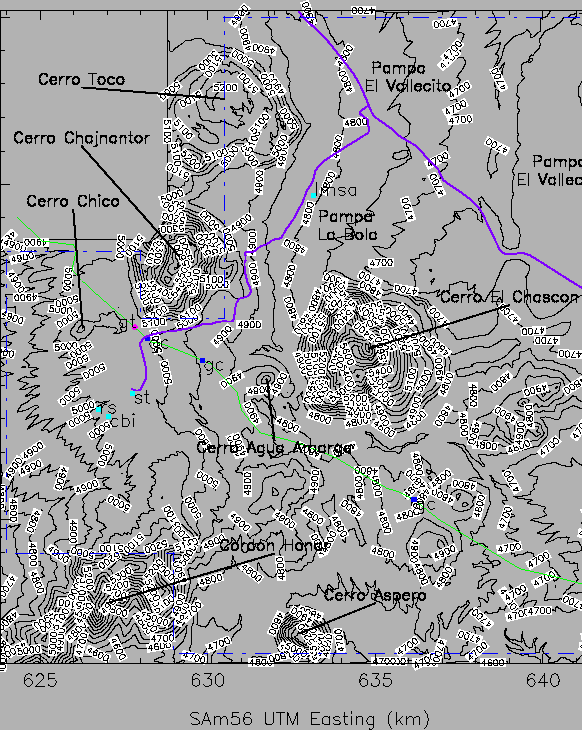
In this memo we consider the entire area for which we have high resolution digital maps, which encompasses the entire extent of the current science preserve. This study area is roughly bounded by UTM coordinates 624000 - 642000 E and 7446000 - 7465000 N (SAm56 datum; Radford 1999). Figure 1 shows the study area, along with the topography (taken from the work of Holdaway et al. [1996] and recent extensions of that work), and some landmarks. Included in this area is the so-called ``Chajnantor'' area - south of Cerro Chajnantor and west of Cerro Chascon, and the so-called ``Pampa La Bola'' area - east of Cerro Toco and north of Cerro Chascon. The Chajnantor area has been extensively studied by both NRAO and ESO for several years now (Radford & Holdaway 1998; Otárola et al. 1998). The Pampa La Bola area has been studied by the NRO for several years (Ishiguro 1998). Also included in this area is the so-called ``Pampa El Vallecito'' area - north and northeast of Cerro Chascon. We have little qualitative and no quantitative information on this area.
 |
In choosing the location of the compact configuration, many things must be considered, including accessibility, thickness of surface weathering layer, proximity to the gas pipeline, shadowing by nearby volcanic peaks, local terrain (including slope and roughness), and astronomical quality of the site (e.g., weather, opacity, and phase stability). Most of the locations in the study area are equally easily accessible, so we do not consider that as a limiting constraint. We only currently have limited information on the how the weathering layer thickness varies with location within the study region (see the NRO-NRAO Geotechnical Report in LMSA memo 2000-04), so we do not treat that consideration further here. We note, however, that the thickness of the weathering layer may have a large impact on construction cost, and so a more complete study of both the variation of the thickness of the weathering layer across the entire science preserve, and its impact on construction cost is needed. We exclude from consideration areas which are too close to the boundary of the science preserve. We take 100 m as an acceptable distance from the boundary, but no closer. We now treat each of the other considerations separately.
The Gas Atacama (GA) pipeline cuts through our study area from the southeast to the northwest. The current agreement with GA is to not build within 400 m of the pipeline. Therefore, locations in the study area closer to the pipeline than this were excluded from consideration for the compact configuration. There is another gas pipeline (built by Norandino) which runs approximately parallel to the Jama highway. There is no formal agreement with respect to building next to this pipeline (or the Jama highway for that matter), but we consider that there should be a similar distance from that pipeline to any antennas. We have no good coordinates for that pipeline, so we use rough coordinates for the Jama highway as a proxy for the pipeline coordinates (provided by S. Sakamoto).
The study area is surrounded by tall volcanic peaks, which will
provide obstacles to observing astronomical objects at low elevations
(and particular azimuths). We have calculated the shadowing at every
location in the study area due to all other locations in the area.
Not allowing areas which are shadowed by 15![]() or more (which we
consider a sensible limit) excludes a significant portion of the study
area from consideration for the location of the compact configuration.
Figure 2 shows the 15
or more (which we
consider a sensible limit) excludes a significant portion of the study
area from consideration for the location of the compact configuration.
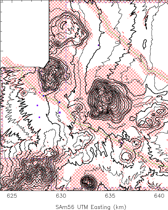
Figure 2 shows the 15![]() shadow regions from these peaks
as colored areas on the topographic map, as well as the areas excluded
because of proximity to the gas pipeline. Also included in
Figure 2 are areas which are outside the science preserve, and
those within 100 m of its boundary. One could argue that the shadowing
constraint should be azimuthally dependent - because shadowing to the
north is more critical than in other directions. This is probably
valid when addressing questions of where to place individual antennas
for the more extended configurations, but we feel that the stricter
constraint is more appropriate when considering the position of the
entire compact configuration.
shadow regions from these peaks
as colored areas on the topographic map, as well as the areas excluded
because of proximity to the gas pipeline. Also included in
Figure 2 are areas which are outside the science preserve, and
those within 100 m of its boundary. One could argue that the shadowing
constraint should be azimuthally dependent - because shadowing to the
north is more critical than in other directions. This is probably
valid when addressing questions of where to place individual antennas
for the more extended configurations, but we feel that the stricter
constraint is more appropriate when considering the position of the
entire compact configuration.
 |
We should place the compact configuration in a place that is ``smooth'' and ``flat'', if possible. These terms are somewhat vague, but in practice this can be achieved by minimizing slope and roughness in the region where the compact configuration will be located. Places that are too steep or too rough will make construction more difficult and hence more costly.
We use here the surface tilt angle as a measure of slope. We define
the surface tilt angle as the deviation from vertical of the normal
of the best-fit plane to the points within a given radius of the
location under consideration. We define the roughness as the rms
deviation of the surface heights after the removal of that best-fit
plane. The size of the regions we are considering here is 200 m
(diameter), which is most likely somewhat larger than the compact
configuration (the compact configuration is about 150 m in diameter for
64 12 m diameter antennas with 40% filling factor), but allows some
room for outlying structures, roads, turnouts, etc... (if needed).
Note that over 200 m, a 1![]() tilt angle results in about 3.5 m of
relief. So, we would like the tilt angle to be
tilt angle results in about 3.5 m of
relief. So, we would like the tilt angle to be
![]() a few degrees.
We would probably like the rms roughness to be less than a meter or so,
if possible. These two limits are somewhat arbitrary, but are based on
the possibility of having to excavate into solid bedrock if the tilt
angles or rms roughness are too large. Depths to solid bedrock as
shallow as 1.6 m were encountered when drilling a number of
boreholes - see Table 2 of the NRO-NRAO Geotechnical Report in LMSA
memo 2000-04. Note, however, that if the cost of excavating into solid
bedrock (and earth-moving in general) are very small, then we could
allow for regions with larger tilts and roughnesses. We currently have
no real estimates for these costs, so we have taken a conservative
approach in this respect. Figure 3 shows a plot of the
derived tilt angles over the entire study area, in 200 m diameter
areas. In this figure, the regions with tilt angles less than
2
a few degrees.
We would probably like the rms roughness to be less than a meter or so,
if possible. These two limits are somewhat arbitrary, but are based on
the possibility of having to excavate into solid bedrock if the tilt
angles or rms roughness are too large. Depths to solid bedrock as
shallow as 1.6 m were encountered when drilling a number of
boreholes - see Table 2 of the NRO-NRAO Geotechnical Report in LMSA
memo 2000-04. Note, however, that if the cost of excavating into solid
bedrock (and earth-moving in general) are very small, then we could
allow for regions with larger tilts and roughnesses. We currently have
no real estimates for these costs, so we have taken a conservative
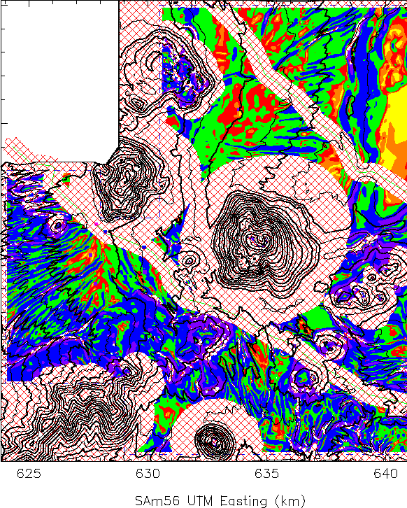
approach in this respect. Figure 3 shows a plot of the
derived tilt angles over the entire study area, in 200 m diameter
areas. In this figure, the regions with tilt angles less than
2![]() are colored red, orange, and yellow, and are the regions of
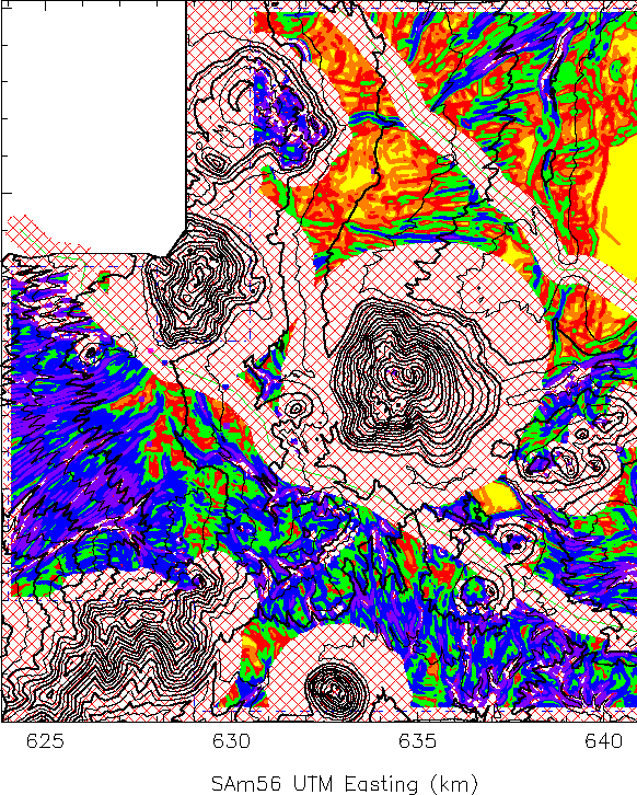
interest. Figure 4 shows a plot of the derived rms roughness
over the entire study area, in 200 m areas. In this figure, the
regions with rms roughness less than 1 m are colored red, orange, and
yellow, and are again the regions of interest.
are colored red, orange, and yellow, and are the regions of
interest. Figure 4 shows a plot of the derived rms roughness
over the entire study area, in 200 m areas. In this figure, the
regions with rms roughness less than 1 m are colored red, orange, and
yellow, and are again the regions of interest.
 |
 |
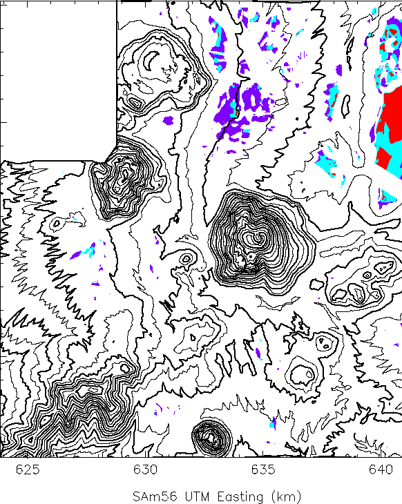
We consider three combinations of maximum surface tilt angle and rms
roughness: 0.5![]() tilt angle and 0.25 m roughness; 1
tilt angle and 0.25 m roughness; 1![]() tilt
angle and 0.5 m roughness; and 2
tilt
angle and 0.5 m roughness; and 2![]() tilt angle and 0.5 m roughness.
Figure 5 shows the centers of the areas that satisfy these
constraints and also are not in the areas which are prohibited by
proximity to the science preserve boundary, gas pipeline, or volcanic
peaks.
tilt angle and 0.5 m roughness.
Figure 5 shows the centers of the areas that satisfy these
constraints and also are not in the areas which are prohibited by
proximity to the science preserve boundary, gas pipeline, or volcanic
peaks.
 |
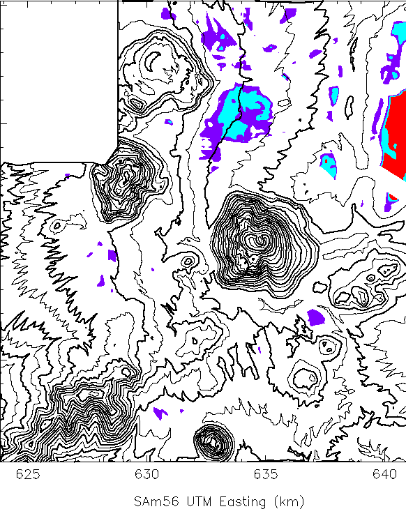
Are there even larger regions which are relatively smooth and flat?
This is of interest because it would be nice to be able to put the
larger configurations in the same place (the next configuration size is
of order 450 m). We went through the same exercise for 500 m regions
and found the regions which are the smoothest and flattest in the study
area on this scale. The only regions which satisfy the same criteria
as for the 200 m regions which are plotted in Figure 5 are in
the Pampa El Vallecito area. If we loosen the criteria somewhat, then
regions in Pampa La Bola and finally in Chajnantor begin to satisfy
these slightly relaxed criteria. Figure 6 shows these areas
which satisfy constraints of 1![]() tilt angle and 0.5 m roughness,
2
tilt angle and 0.5 m roughness,
2![]() tilt angle and 1 m roughness, and 3
tilt angle and 1 m roughness, and 3![]() tilt angle and
1.5 m roughness.
tilt angle and
1.5 m roughness.
 |
We would like to know how the astronomical quality varies from place to place across the entire study area in detail. A rough indicator of this may be obtained from surface weather data. The analysis of several years of weather data (including wind, temperature, relative humidity, and solar flux) obtained at Chajnantor and Pampa La Bola indicates that while there are differences between the two sites, these differences are not significant enough to seriously influence a decision on which is the ``better'' astronomical site (Sakamoto et al. 2000). Much better indicators of the astronomical quality are the atmospheric opacity and phase stability. These two quantities have been measured at the locations of the site testing containers (at least sporadically) over several years now. A preliminary analysis of a small amount of phase stability data (from Jul-Sep 1996) from the NRAO and NRO container locations showed that the Pampa La Bola site was slightly worse in phase stability than the Chajnantor site (Holdaway et al. 1997). It has been postulated that this is due to local turbulence caused by the wind as it rises up over Cerros Chajnantor and Toco. This has yet to be shown conclusively, however, and a more complete comparison of both the phase stability and opacity data from the two locations is needed. We have no data for sites further to the east (e.g., Pampa El Vallecito) and thus no comparisons are possible. We can say crudely that we expect the opacity to be worse at lower elevations (and hence Chajnantor to be best, followed by Pampa La Bola, and finally Pampa El Vallecito), but without data, this is not quantifiable. Until a good comparison of site testing data is made, and one or the other site shown to be clearly better than the other, it seems somewhat hasty to exclude any site from consideration based on this criterion.
There are locations in both the Chajnantor and Pampa La Bola areas which are good candidates for the location of the compact ALMA configuration. There is also a very large region in Pampa El Vallecito which might be a good candidate for that location. Without any data in hand to evaluate the Pampa El Vallecito area, however, it seems that it will be hard to justify selection of this area for the location of the compact ALMA configuration. Table 1 shows all of the locations, along with an indicator of their ``quality'', in terms of flatness, roughness, and extent. Note that there are so many good locations in Pampa La Bola that we have not attempted to make an extensive tabulation of them, but merely put the best one in the table. Also note that in the Chajnantor area, the preferred locations are mostly along the high ridge in the western portion of the area. Table 1 also shows the proposed centers of the compact configurations in the two current strawperson configurations (Yun & Kogan 2000; Conway 2000) for comparison.
|
SAm56 UTM Easting |
SAm56 UTM Northing | elevation (m) | location | quality |
|
627650 |
7454450 | 5030 | Chajnantor | best |
| 627750 | 7453100 | 5030 | Chajnantor | better |
| 628050 | 7453650 | 5025 | Chajnantor | better |
| 630400 | 7453550 | 4912 | Chajnantor | good |
| 633800 | 7460600 | 4801 | Pampa La Bola | best |
| 640700 | 7459400 | 4609 | Pampa El Vallecito | best |
| 628370 | 7453250 | 5013 | Donut | -- |
| 628590 | 7454000 | 5013 | Zoom | -- |
|
|
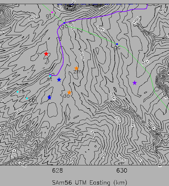
We note that the selection of the location of the compact configuration may have serious implications for the configuration designs, as designs with self-similarity (the ``zoom'' configurations - e.g., Conway 2000), have the compact configuration near the center of the geometry (spirals, circles, or triangles) whereas the more traditional fixed designs (e.g., Yun & Kogan 2000) do not necessarily. The best locations for the compact configuration in the Chajnantor area we suggest here may not allow for zoom configurations, as there may be no room for a 3-5 km configuration to be designed with those centers. This deserves more study. Figure 7 shows visually how the locations in the current configuration designs compare with the ones determined here for the Chajnantor area.
 |
We emphasize lastly that the final selection of the location for the compact configuration will certainly be influenced by more factors than we have considered here, including the political viability of the various sites when considered as a whole. In addition, the comparison of the opacity and phase stability data from the Chajnantor and Pampa La Bola site testing locations is of vital importance in making a decision as to the best location for the compact configuration.
Conway, J.E., A Possible Layout for a Spiral Zoom Array Incorporating Terrain Constraints, ALMA Memo. No. 292, 2000
Holdaway, M.A., S. Matsushita, & M. Saito, Preliminary Phase Stability Comparison of the Chajnantor and Pampa la Bola sites, MMA Memo. No. 176, 1997
Holdaway, M.A., M.A. Gordon, S.M. Foster, F.R. Schwab, & H. Bustos, Digital Elevation Models for the Chajnantor Site, MMA Memo. No. 160, 1996
Ishiguro, M., Japanese Large Millimeter and Submillimeter Array, Proc. SPIE, 3357, 244-253, 1998
Otárola, A., and 9 others, European Site Testing at Chajnantor: a Step Towards the Large Southern Array, ESO Messenger, 94, 13-20, 1998
Radford, S.J.E., Position of MMA Equipment on Chajnantor, MMA Memo. No. 261, 1999
Radford, S.J.E., & M.A. Holdaway, Atmospheric conditions at a site for submillimeter wavelength astronomy, Proc. SPIE, 3357, 486-494, 1998
Sakamoto, S., and 7 others, Comparison of Meteorological Data at the Pampa La Bola and Llano de Chajnantor Sites, ALMA Memo. No. 322, 2000
Yun, M.S., & L. Kogan, Strawperson Donut/Doubling-Ring Configurations, ALMA Memo. No. 320, 2000
This document was generated using the LaTeX2HTML translator Version 99.2beta8 (1.42)
Copyright © 1993, 1994, 1995, 1996,
Nikos Drakos,
Computer Based Learning Unit, University of Leeds.
Copyright © 1997, 1998, 1999,
Ross Moore,
Mathematics Department, Macquarie University, Sydney.
The command line arguments were:
latex2html -split 0 -no_navigation small
The translation was initiated by Bryan Butler on 2000-12-04