Radiometric Phase Correction
C.L. Carilli
National Radio Astronomy Observatory
Socorro, NM, 87801
ccarilli@nrao.edu
O. Lay
University of California at Berkeley
Radio Astronomy Laboratory
Berkeley, CA, 94720
olay@astron.berkeley.edu
E.C. Sutton
University of Illinois
Department of Astronomy
Urbana, IL, 61801
sutton@astro.uiuc.edu
January 15, 1998
We analyze the technique of using radiometers to measure
the precipitable water vapor (PWV) content of the atmosphere in
order to correct interferometric data for
phase noise due PWV fluctuations in the troposphere.
We present an idealized
model of phase fluctuations due to PWV variations in the troposphere
based on the Taylor hypothesis, and we summarize the radiometry
equations. We then consider various options for radiometric phase
corrections, including:
(i) the very demanding technique of making an absolute measurement
of PWV at each antenna assuming an accurate (absolutely calibrated)
measurement of brightness temperature, T![]() , and using a theoretical
model for the troposphere and measured physical parameters for
the troposphere (temperature, pressure, etc...), and (ii)
the less demanding technique of using a strong celestial calibration source
to derive an empirical relationship between brightness temperature
fluctuations and atmospheric phase fluctuations.
, and using a theoretical
model for the troposphere and measured physical parameters for
the troposphere (temperature, pressure, etc...), and (ii)
the less demanding technique of using a strong celestial calibration source
to derive an empirical relationship between brightness temperature
fluctuations and atmospheric phase fluctuations.
Radiometric phase correction requires systems that
are sensitive (19 ![]() T
T![]()
![]() 920 mK), and
stable over long timescales (200
920 mK), and
stable over long timescales (200 ![]()
![]() Gain
Gain ![]() 15000).
Absolute radiometric phase correction at each antenna also requires
knowledge of the tropospheric parameters, such as
T
15000).
Absolute radiometric phase correction at each antenna also requires
knowledge of the tropospheric parameters, such as
T![]() , P
, P![]() , and h
, and h![]() , to a few percent or less.
And even if such accurate measurements are available, fundamental
uncertainties in the atmospheric models relating T
, to a few percent or less.
And even if such accurate measurements are available, fundamental
uncertainties in the atmospheric models relating T![]() and PWV may
require empirical calibration of the T
and PWV may
require empirical calibration of the T![]() - w
- w![]() relationship at regular intervals.
relationship at regular intervals.
The empirical approach increases the coherence time of the array, but a
number questions remain to be answered, including:
(i) over what time scale and distance will this technique allow
for radiometric phase corrections when switching between
the source and the calibrator?, and
(ii) how often will calibration of the T![]() -
- ![]() relationship be required, ie. how stable are the mean parameters of
the atmosphere?
relationship be required, ie. how stable are the mean parameters of
the atmosphere?
The radiometry equation (Dicke et al. 1946) relates the observed brightness
temperature of the sky, T![]() , to the atmospheric temperature,
T
, to the atmospheric temperature,
T![]() , and the total optical depth through the atmosphere,
, and the total optical depth through the atmosphere,
![]() , as:
, as:
![]()
The opacity is due to the pressure broadened wings of various
mm, sub-mm, and IR lines of water vapor, O![]() , and other trace gases
(CO,N
, and other trace gases
(CO,N![]() O,...). The contribution
from O
O,...). The contribution
from O![]() and other trace gases is thought to be stable over
time. The water vapor contribution can be time variable.
This has led to the hypothesis that
by measuring fluctuations in T
and other trace gases is thought to be stable over
time. The water vapor contribution can be time variable.
This has led to the hypothesis that
by measuring fluctuations in T![]() with a radiometer, one can derive
the fluctuations in the column density of water vapor of the troposphere
(Barrett and Chung 1962, Staelin 1966, Westwater and Guiraud
1980, Rosenkranz 1989). This column density is usually quantified in
terms of the effective depth of water vapor converted to the liquid
phase: w = milli-meters of precipitable water vapor (PWV).
with a radiometer, one can derive
the fluctuations in the column density of water vapor of the troposphere
(Barrett and Chung 1962, Staelin 1966, Westwater and Guiraud
1980, Rosenkranz 1989). This column density is usually quantified in
terms of the effective depth of water vapor converted to the liquid
phase: w = milli-meters of precipitable water vapor (PWV).
Water vapor affects the index of refraction of the troposphere, hence variations in PWV lead to variations in the effective electrical path length, corresponding to variations in the phase of a electromagnetic wave propagating through the troposphere (Tatarskii 1978). Such variations are seen as `phase noise' by radio interferometers. Since the effect increases linearly with frequency (except in the vicinity of the strong water lines), such variations are most prominent for mm and sub-mm interferometers, and phase variations caused by tropospheric PWV fluctuations can be the limiting factor for the coherence time and spatial resolution of mm interferometers (Hinder and Ryle 1971).
Many groups have proposed to reduce tropospheric phase variations by
measuring fluctuations in PWV using radiometers
(Resch, Hogg, and Napier 1984, Bagri 1994, Woody and Marvel 1998).
The correlation
between T![]() and interferometer phase has been demonstrated by a
number of groups (Bagri 1994, Resch, Hogg, and Napier 1984). However,
the conversion of these values
to antenna-based electrical phase, and the subsequent application of
these phases to interferometric data, has met with mixed success
(Welch 1994, Bremer, Guilloteau, and Lucas, R. 1997).
and interferometer phase has been demonstrated by a
number of groups (Bagri 1994, Resch, Hogg, and Napier 1984). However,
the conversion of these values
to antenna-based electrical phase, and the subsequent application of
these phases to interferometric data, has met with mixed success
(Welch 1994, Bremer, Guilloteau, and Lucas, R. 1997).
In this memorandum we investigate the technique of using radiometers to reduce tropospheric phase fluctuations, both in the context of the MMA site at Chajnantor, and at the VLA site. We present an idealized model of phase fluctuations due to PWV variations in the troposphere based on the Taylor hypothesis. We then summarize the radiometry equations, and we consider various options for radiometric phase corrections. We begin by considering the very stringent requirement of making an absolute measurement of PWV at each antenna assuming an accurate (absolutely calibrated) measurement of brightness temperature, and using a theoretical model for the troposphere and measured physical parameters for the troposphere (temperature, pressure, etc...). We then consider the less demanding technique of using a strong celestial calibration source to derive an empirical relationship between brightness temperature fluctuations and atmospheric phase fluctuations at regular intervals.
The standard model for tropospheric phase
fluctuations involves variations
in the water vapor column density
in a turbulent layer in the troposphere with
a mean height, h![]() , and a vertical extent, W, which
moves at some velocity, V
, and a vertical extent, W, which
moves at some velocity, V![]() .
This model includes the `Taylor hypothesis', or `frozen screen
approximation', which states that: `if the turbulent intensity
is low and the turbulence is approximately stationary and homogeneous,
then the turbulent field is unchanged over the atmospheric boundary
layer time scales of interest and advected with the mean wind'
(Taylor 1938, Garratt 1992).
Under this assumption one can relate temporal and spatial
phase fluctuations with a simple Eulerian transformation
using V
.
This model includes the `Taylor hypothesis', or `frozen screen
approximation', which states that: `if the turbulent intensity
is low and the turbulence is approximately stationary and homogeneous,
then the turbulent field is unchanged over the atmospheric boundary
layer time scales of interest and advected with the mean wind'
(Taylor 1938, Garratt 1992).
Under this assumption one can relate temporal and spatial
phase fluctuations with a simple Eulerian transformation
using V![]() . In the following sections we adopt a value of
V
. In the following sections we adopt a value of
V![]() = 10 m s
= 10 m s![]() .
.
Tropospheric phase fluctuations are usually
characterized by a root phase structure function,
![]() (b), equal to the root mean square phase variations on
baselines of length b, when calculated over a sufficiently long time
(time >> baseline crossing time =
(b), equal to the root mean square phase variations on
baselines of length b, when calculated over a sufficiently long time
(time >> baseline crossing time = ![]() ),
or for an ensemble of measurements at a given
time on many baselines of length b. Kolmogorov
turbulence theory (Coulman 1990) predicts a function of the form:
),
or for an ensemble of measurements at a given
time on many baselines of length b. Kolmogorov
turbulence theory (Coulman 1990) predicts a function of the form:
![]()
where b is in km, and ![]() is in mm. In this report we adopt a
typical value of K = 100 for the MMA site in Chajnantor, and K = 300
for the VLA site (Carilli, Holdaway, and Sowinski 1996).
is in mm. In this report we adopt a
typical value of K = 100 for the MMA site in Chajnantor, and K = 300
for the VLA site (Carilli, Holdaway, and Sowinski 1996).
Kolmogorov turbulence theory predicts
n = ![]() for baselines longer than W,
and n =
for baselines longer than W,
and n = ![]() for baselines
shorter than W (Coulman 1990). The change in power-law index at b = W is
due to the finite vertical extent
of the turbulent layer. For baselines
shorter than the typical turbulent layer extent the full 3-dimensionality
of the turbulence is involved (thick-screen), while for longer baselines
a 2-dimensional approximation applies (thin-screen).
Turbulence theory also predicts an `outer-scale', L
for baselines
shorter than W (Coulman 1990). The change in power-law index at b = W is
due to the finite vertical extent
of the turbulent layer. For baselines
shorter than the typical turbulent layer extent the full 3-dimensionality
of the turbulence is involved (thick-screen), while for longer baselines
a 2-dimensional approximation applies (thin-screen).
Turbulence theory also predicts an `outer-scale', L![]() , beyond which the
rms phase should no increase with baseline length
(ie. n = 0). This scale corresponds to
the largest coherent structures, or maximum correlation length,
for water vapor fluctuations in the troposphere, presumably set by
external boundary conditions.
, beyond which the
rms phase should no increase with baseline length
(ie. n = 0). This scale corresponds to
the largest coherent structures, or maximum correlation length,
for water vapor fluctuations in the troposphere, presumably set by
external boundary conditions.
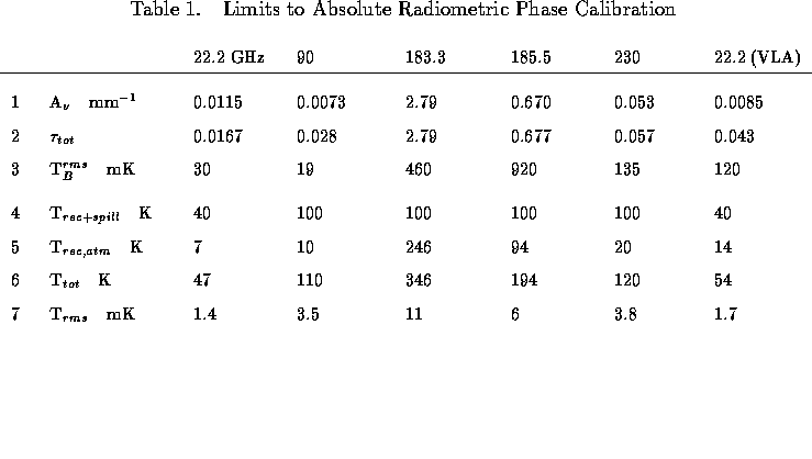
Recent observations with the VLA by Carilli and Holdaway (1997)
support Kolmogorov theory for tropospheric phase fluctuations.
Their result is reproduced in Figure 1,
which shows the root phase structure function made using the BnA
configuration of the VLA. This configuration has good baseline
coverage ranging from 200m to 20 km, hence sampling all three
hypothesized ranges in the structure function.
Observations were made during the night of Jan. 27, 1997 using
the VLA calibration source 0748+240. The total observing time was 90
min, corresponding to a tropospheric travel distance of 54 km, assuming
V![]() = 10 m s
= 10 m s![]() .
The open circles show the nominal tropospheric root phase structure
function over the full 90 min time range. The
solid squares are the rms phases after subtracting (in
quadrature) a constant electronic noise term of 10
.
The open circles show the nominal tropospheric root phase structure
function over the full 90 min time range. The
solid squares are the rms phases after subtracting (in
quadrature) a constant electronic noise term of 10![]() , as derived from
the data by requiring the best power-law on short baselines.
The 10
, as derived from
the data by requiring the best power-law on short baselines.
The 10![]() noise term is consistent with previous measurements at the
VLA indicating electronic phase noise increasing with frequency as
0.5
noise term is consistent with previous measurements at the
VLA indicating electronic phase noise increasing with frequency as
0.5![]() per GHz (Carilli and Holdaway 1996).
per GHz (Carilli and Holdaway 1996).
The three regimes of the structure function as predicted
by Kolmogorov theory are verified in Figure 1.
On short baselines (b ![]() 1.2 km) the measured power-law index
is 0.85
1.2 km) the measured power-law index
is 0.85![]() 0.03 and the predicted value is 0.83. On intermediate
baselines (1.2
0.03 and the predicted value is 0.83. On intermediate
baselines (1.2 ![]() b
b ![]() 6 km)
the measured index is 0.41
6 km)
the measured index is 0.41![]() 0.03 and the predicted value
is 0.33. On long baselines (b
0.03 and the predicted value
is 0.33. On long baselines (b ![]() 6 km) the measured index is
0.1
6 km) the measured index is
0.1![]() 0.2 and the predicted value is zero. The implication is that
the vertical extent of the turbulent layer is: W
0.2 and the predicted value is zero. The implication is that
the vertical extent of the turbulent layer is: W
![]() 1 km, and that the outer scale of the turbulence is:
L
1 km, and that the outer scale of the turbulence is:
L![]()
![]() 6 km. The increase in the scatter of the rms phases
for baselines longer than
6 km may be due to an anisotropic outer scale (see Carilli and
Holdaway 1997).
6 km. The increase in the scatter of the rms phases
for baselines longer than
6 km may be due to an anisotropic outer scale (see Carilli and
Holdaway 1997).
A rigorous treatment of the radiometry equation (1) involves
integration of the radiative transfer equations
through the atmosphere using the vertical profiles of
temperature and density, and using models for the spectral line shapes.
There are number of codes which generate
synthetic atmospheric optical depth and T![]() spectra using extensive
lists of spectral lines from atmospheric constituents under various
conditions (Liebe 1989, Sutton and Hueckstaedt 1997). One well known
problem with these models is that they substantially
under-predict T
spectra using extensive
lists of spectral lines from atmospheric constituents under various
conditions (Liebe 1989, Sutton and Hueckstaedt 1997). One well known
problem with these models is that they substantially
under-predict T![]() for a given amount of PWV, in particular for
measurements made away from the water lines. The likely cause of this
discrepancy is incorrect line shapes far into the wings of the lines
(Sutton and Hueckstaedt 1997). Hence, many codes also include
empirically determined `water vapor continuum
fudge-factors' to mitigate this discrepancy. If this discrepancy is
due to incorrect line shapes, then these fudge-factors may be
functions of both atmospheric pressure and temperature, and hence are
likely to be time variable (section 5).
for a given amount of PWV, in particular for
measurements made away from the water lines. The likely cause of this
discrepancy is incorrect line shapes far into the wings of the lines
(Sutton and Hueckstaedt 1997). Hence, many codes also include
empirically determined `water vapor continuum
fudge-factors' to mitigate this discrepancy. If this discrepancy is
due to incorrect line shapes, then these fudge-factors may be
functions of both atmospheric pressure and temperature, and hence are
likely to be time variable (section 5).
For the purposes of the calculations presented herein we have used the
atmospheric model of Liebe (1989), as maintained by
Holdaway and Pardo (1997). This model includes a local
line base of 44 O![]() lines plus 30 H
lines plus 30 H![]() O lines plus
lines from trace gases in the range from 20 GHz to 1000 GHz, and
an empirical (power-law) correction for the `water vapor continuum'.
The code employs the U.S. Standard Model Atmosphere,
for which the ground temperature and pressure at the MMA site are:
270 K and 560 mb, respectively. The corresponding values for
the VLA site are: 287 K and 790 mb. A linear gradient of temperature
with elevation of -6 K km
O lines plus
lines from trace gases in the range from 20 GHz to 1000 GHz, and
an empirical (power-law) correction for the `water vapor continuum'.
The code employs the U.S. Standard Model Atmosphere,
for which the ground temperature and pressure at the MMA site are:
270 K and 560 mb, respectively. The corresponding values for
the VLA site are: 287 K and 790 mb. A linear gradient of temperature
with elevation of -6 K km![]() is assumed.
is assumed.
For the MMA the site elevation is 5000 m
(Chajnantor), and the typical optical depth at 230 GHz is 0.06, implying
a mean w = 1 mm (Holdaway and Pardo 1997).
For the VLA the site elevation is 2150 m and the typical opacity at
43 GHz is 0.06, implying a mean w = 5 mm.
Plots of the atmospheric T![]() and transmission for the MMA and VLA
sites under these assumptions are shown in Figures 2 and 3, for
frequencies ranging from 0 to 1000 GHz. Figures 4 and 5 are blow-ups
of the optical depth from 0 to 250 GHz, with the different components
(PWV and other gases) shown explicitly.
and transmission for the MMA and VLA
sites under these assumptions are shown in Figures 2 and 3, for
frequencies ranging from 0 to 1000 GHz. Figures 4 and 5 are blow-ups
of the optical depth from 0 to 250 GHz, with the different components
(PWV and other gases) shown explicitly.
We assume that the atmospheric opacity can be divided into three parts:
![]()
where: (i) A![]() is the
optical depth per mm of PWV (Figures 4 and
5) as a function of frequency,
(ii) w
is the
optical depth per mm of PWV (Figures 4 and
5) as a function of frequency,
(ii) w![]() is the temporally stable (mean)
value for PWV of the troposphere, (iii) B
is the temporally stable (mean)
value for PWV of the troposphere, (iii) B![]() is the total
optical depth due to all other gases besides water as
a function of frequency (also assumed to be
temporally stable), and (iv) w
is the total
optical depth due to all other gases besides water as
a function of frequency (also assumed to be
temporally stable), and (iv) w![]() is the time variable component
of the PWV of the troposphere. It is this time variable component which
causes the tropospheric phase `noise' for an interferometer.
In effect, we assume a constant mean optical depth:
is the time variable component
of the PWV of the troposphere. It is this time variable component which
causes the tropospheric phase `noise' for an interferometer.
In effect, we assume a constant mean optical depth: ![]() , with a fluctuating term due to changes
in PWV:
, with a fluctuating term due to changes
in PWV: ![]() , and that
, and that
![]() >>
>> ![]() .
.
Inserting (3) into equation (1), and making the reasonable assumption
that A![]()
![]() w
w![]() , leads to:
, leads to:
![]()
The first term on the righthand side of equation (4) represents the
mean, non-varying T![]() of the troposphere. The second term represents
the fluctuating component due to variations in PWV, which we define
as:
of the troposphere. The second term represents
the fluctuating component due to variations in PWV, which we define
as:
![]()
At first glance, it would appear that equation (5) applies to
fluctuations in a turbulent layer at the top of the
troposphere, since the fluctuating component is fully attenuated
(ie. multiplied by ![]() ). However, for a turbulent
layer at lower altitudes there is the additional term of attenuation
of the atmosphere above the turbulent layer by the turbulence.
It can be shown that the terms exactly cancel for an isobaric,
isothermal atmosphere, in which case
equation 5 is independent of the height of the turbulence.
). However, for a turbulent
layer at lower altitudes there is the additional term of attenuation
of the atmosphere above the turbulent layer by the turbulence.
It can be shown that the terms exactly cancel for an isobaric,
isothermal atmosphere, in which case
equation 5 is independent of the height of the turbulence.
We can then use the relationships between w and electrical pathlength
to derive the phase fluctuations due to the troposphere.
The electrical pathlength, L, is given by: L![]() 6.5
6.5![]() w,
across most of the mm to sub-mm spectrum, except in the vicinity of
the strong water lines where dispersive effects become
significant (Hogg, Guiraud, and Decker 1981). The extra phase,
w,
across most of the mm to sub-mm spectrum, except in the vicinity of
the strong water lines where dispersive effects become
significant (Hogg, Guiraud, and Decker 1981). The extra phase, ![]() ,
introduced to a propagating electromagnetic wave is then:
,
introduced to a propagating electromagnetic wave is then:
![]()
The absolute radiometric phase correction process entails measuring
variations in brightness temperature
(T![]() ) with a radiometer, inverting equation (5) to
derive the variation in PWV (w
) with a radiometer, inverting equation (5) to
derive the variation in PWV (w![]() ), and then using equation (6)
to derive the variation in electronic phase,
), and then using equation (6)
to derive the variation in electronic phase, ![]() , along a
given line of sight.
, along a
given line of sight.
As benchmark numbers for the MMA we set the requirement that we
need to measure changes in tropospheric induced phase above a given
antenna to an accuracy of ![]() at 230 GHz at the
zenith, or
at 230 GHz at the
zenith, or ![]() = 18
= 18![]() . This
requirement inserted into equation (6) then yeilds a required
accuracy of: w
. This
requirement inserted into equation (6) then yeilds a required
accuracy of: w![]() = 0.01 mm.
This value of w
= 0.01 mm.
This value of w![]() then sets the required sensitivity,
T
then sets the required sensitivity,
T![]() , of the
radiometers as a function of frequency through equation 5. For the VLA
we set the
, of the
radiometers as a function of frequency through equation 5. For the VLA
we set the ![]() requirement at 43 GHz, leading to: w
requirement at 43 GHz, leading to: w![]() = 0.05 mm.
In its purest form, the inversion of equation (5) requires: (i) a
sensitive, absolutely calibrated radiometer, (ii) accurate
values for the run of temperature and pressure as a function of
height in the atmosphere, and (iii) an accurate value for the height
of the PWV fluctuations. We consider the requirements on each
of these terms in detail in section 5.
= 0.05 mm.
In its purest form, the inversion of equation (5) requires: (i) a
sensitive, absolutely calibrated radiometer, (ii) accurate
values for the run of temperature and pressure as a function of
height in the atmosphere, and (iii) an accurate value for the height
of the PWV fluctuations. We consider the requirements on each
of these terms in detail in section 5.
Figure 6 shows the required sensitivity of the radiometer,
T![]() , given the benchmark numbers for w
, given the benchmark numbers for w![]() for the VLA and
the MMA and using equation (5). It is important to keep in mind that
lower numbers on this plot imply that more sensitive radiometry is required
in order to measure the benchmark value of w
for the VLA and
the MMA and using equation (5). It is important to keep in mind that
lower numbers on this plot imply that more sensitive radiometry is required
in order to measure the benchmark value of w![]() .
Figure 7 shows the detailed behavior of atmospheric brightness
temperature, atmospheric transmission, and T
.
Figure 7 shows the detailed behavior of atmospheric brightness
temperature, atmospheric transmission, and T![]() in the
vicinity of the water lines at
22.2 GHZ and 183.3 GHz. The required T
in the
vicinity of the water lines at
22.2 GHZ and 183.3 GHz. The required T![]() values generally
increase with increasing frequency due to the increase in A
values generally
increase with increasing frequency due to the increase in A![]() ,
with a local maximum at the 22 GHz water line,
and minima at the strong O
,
with a local maximum at the 22 GHz water line,
and minima at the strong O![]() lines (59.2 GHz and 118.8 GHz).
The strong water line at 183.3 GHz shows
a `double peak' profile, with a local minimum in T
lines (59.2 GHz and 118.8 GHz).
The strong water line at 183.3 GHz shows
a `double peak' profile, with a local minimum in T![]() at the
frequency corresponding to the peak T
at the
frequency corresponding to the peak T![]() of the line. This behavior
is due to the product: A
of the line. This behavior
is due to the product: A![]()
![]() e
e![]() in equation 5.
The value of A
in equation 5.
The value of A![]() peaks at the line frequency, but this is
off-set by the high total optical depth at the line peak.
This effect is most dramatic for the VLA case,
where the required T
peaks at the line frequency, but this is
off-set by the high total optical depth at the line peak.
This effect is most dramatic for the VLA case,
where the required T![]() at the 183 GHz line peak is very low.
at the 183 GHz line peak is very low.
In this section we consider making an absolute correction to the
electronic phase at a given antenna using an accurate, absolutely
calibrated measurement of T![]() ,
and accurate measurements of tropospheric parameters (temperature and
pressure as a function of height, and the scale height of the PWV
fluctuations). We consider requirements on the gain
stability, sensitivity, and on atmospheric data, given the benchmark
values of w
,
and accurate measurements of tropospheric parameters (temperature and
pressure as a function of height, and the scale height of the PWV
fluctuations). We consider requirements on the gain
stability, sensitivity, and on atmospheric data, given the benchmark
values of w![]() and
using equation (5) to relate w
and
using equation (5) to relate w![]() and T
and T![]() (see Figures 6
- 9). We consider the requirements at a number of frequencies,
including: (i) the water lines at 22.2 GHz and 183.3 GHz, (ii) the
half power of the water line at 185.5 GHz, and (iii) two continuum
bands at 90 GHz and 230 GHz. For the VLA we only consider the 22.2
GHz line.
(see Figures 6
- 9). We consider the requirements at a number of frequencies,
including: (i) the water lines at 22.2 GHz and 183.3 GHz, (ii) the
half power of the water line at 185.5 GHz, and (iii) two continuum
bands at 90 GHz and 230 GHz. For the VLA we only consider the 22.2
GHz line.
The results are summarized in Table 1. Row 1 shows the optical
depth per mm PWV, A![]() , at the different frequencies for the model
atmospheres discussed in section 4, while row 2 shows the total
optical depth,
, at the different frequencies for the model
atmospheres discussed in section 4, while row 2 shows the total
optical depth, ![]() , for the models. Row 3 shows the required
T
, for the models. Row 3 shows the required
T![]() values as derived from equation (5). It is important to
keep in mind that these values are simply the expected change in
T
values as derived from equation (5). It is important to
keep in mind that these values are simply the expected change in
T![]() given a change in w of 0.01 mm for the MMA and 0.05 mm for the
VLA, for a single radiometer looking at the zenith. All subsequent
calculations depend on these basic T
given a change in w of 0.01 mm for the MMA and 0.05 mm for the
VLA, for a single radiometer looking at the zenith. All subsequent
calculations depend on these basic T![]() values. The values range from 19 mK at 90 GHz,
to 920 mK at 185.5 GHz, at the MMA site, and 120 mK for the VLA site
at 22 GHz.
values. The values range from 19 mK at 90 GHz,
to 920 mK at 185.5 GHz, at the MMA site, and 120 mK for the VLA site
at 22 GHz.
We consider sensitivity and gain stability. Row 4 lists
approximate numbers for expected receiver temperatures,
T![]() , in the case of
cooled systems (eg. using the astronomical receivers for radiometry).
Row 5 lists the contribution to the system temperature from the
atmosphere, T
, in the case of
cooled systems (eg. using the astronomical receivers for radiometry).
Row 5 lists the contribution to the system temperature from the
atmosphere, T![]() , and row 6 lists the
expected total system temperature, T
, and row 6 lists the
expected total system temperature, T![]() (sum of row 4 and 5).
Row 7 lists the rms sensitivity of the radiometers, T
(sum of row 4 and 5).
Row 7 lists the rms sensitivity of the radiometers, T![]() , assuming
1000 MHz bandwidth, one polarization, and a 1 sec
integration time. In all cases the expected sensitivities of the
radiometers are well
below the required T
, assuming
1000 MHz bandwidth, one polarization, and a 1 sec
integration time. In all cases the expected sensitivities of the
radiometers are well
below the required T![]() values, indicating that sensitivity
should not be a limiting factor for these systems. Row 8 lists the
required gain stability of the system, defined as the ratio of total system
temperature to T
values, indicating that sensitivity
should not be a limiting factor for these systems. Row 8 lists the
required gain stability of the system, defined as the ratio of total system
temperature to T![]() :
: ![]() Gain
Gain ![]()
![]() . Values range from 210 for the 185.5 GHz
measurement to 5800 for the 90 GHz measurement at the MMA, and 450 for
the VLA site at 22 GHz.
. Values range from 210 for the 185.5 GHz
measurement to 5800 for the 90 GHz measurement at the MMA, and 450 for
the VLA site at 22 GHz.
Rows 9 and 10 list total system temperatures and expect rms
sensitivities in the case of uncooled radiometers.
We adopt a constant total system temperature of
T![]() = 2000 K, but the other parameters remain the same
(bandwidth, etc...). The radiometer sensitivity is then 63 mK in 1 sec.
This sensitivity is adequate
to reach the benchmark T
= 2000 K, but the other parameters remain the same
(bandwidth, etc...). The radiometer sensitivity is then 63 mK in 1 sec.
This sensitivity is adequate
to reach the benchmark T![]() values in row 3, although at 230
GHz the sensitivity value is within a factor two of the required
T
values in row 3, although at 230
GHz the sensitivity value is within a factor two of the required
T![]() . The required gain stabilities in this case are listed in
row 11. The requirement becomes severe at 230 GHz
(
. The required gain stabilities in this case are listed in
row 11. The requirement becomes severe at 230 GHz
(![]() Gain = 15000).
Gain = 15000).
We consider the requirements on atmospheric data, beginning with
T![]() . The dependence of T
. The dependence of T![]() on T
on T![]() comes in
explicitly in equation (5) through the first multiplier, and implicitly
through the effect of T
comes in
explicitly in equation (5) through the first multiplier, and implicitly
through the effect of T![]() on
on ![]() . For simplicity, we
consider only the explicit dependence,
which will lead to an underestimate of the
expected errors by at most a factor
. For simplicity, we
consider only the explicit dependence,
which will lead to an underestimate of the
expected errors by at most a factor ![]() two - adequate for the
purposes of this document (Sutton and
Hueckstaedt 1997). Under this simplifying assumption the required accuracy,
two - adequate for the
purposes of this document (Sutton and
Hueckstaedt 1997). Under this simplifying assumption the required accuracy,
![]() T
T![]() , becomes:
, becomes:
![]()
The values ![]() T
T![]() are listed in row 12. Values in
parentheses are the percentage accuracy in terms of the ground
atmospheric temperature. Values are typically of order 1 K, or a few
tenths of a percent
of the mean. A related requirement is the accuracy of the gradient in
temperature:
are listed in row 12. Values in
parentheses are the percentage accuracy in terms of the ground
atmospheric temperature. Values are typically of order 1 K, or a few
tenths of a percent
of the mean. A related requirement is the accuracy of the gradient in
temperature: ![]()
![]()
![]()
![]() , in
the case of a turbulent layer at h
, in
the case of a turbulent layer at h![]() = 2 km, and
assuming a very accurate measurement of T
= 2 km, and
assuming a very accurate measurement of T![]() on the ground
and a very accurate measurement of h
on the ground
and a very accurate measurement of h![]() .
These values are listed in row 13
of the table. The accuracy requirements range from 0.25 K km
.
These values are listed in row 13
of the table. The accuracy requirements range from 0.25 K km![]() to
1.5 K km
to
1.5 K km![]() , or roughly 10
, or roughly 10![]() of the mean gradient.
Similarly, we can consider the required accuracy of the measurement of
the height of the troposphere,
of the mean gradient.
Similarly, we can consider the required accuracy of the measurement of
the height of the troposphere, ![]() h
h![]()
![]()
![]() ,
assuming a perfect measurement of the ground
temperature and temperature gradient.
These values are listed in row 14. Values are typically a few tenths
of a km, or roughly 10
,
assuming a perfect measurement of the ground
temperature and temperature gradient.
These values are listed in row 14. Values are typically a few tenths
of a km, or roughly 10![]() of h
of h![]() .
.
Finally, we consider the requirements on atmospheric pressure given
the T![]() requirements. The relationship between T
requirements. The relationship between T![]() and w
is affected by atmospheric pressure through the change in the pressure
broadened line shapes. An increase in pressure will transfer power
from the line peak into the line wings, thereby flattening the overall
profile. The expected changes in optical depth (or brightness
temperature) as a function of frequency have been quantified by
Sutton and Hueckstaedt (1997), and their coefficients relating changes
in pressure with changes in optical depth are listed in row 17. Note
the change in sign of the coefficient on the line peaks versus
off-line frequencies. Sutton and Hueckstaedt point out that, since
the integrated power in the line is conserved, there
are `hinge-points' in the line profiles where pressure changes have
very little effect on T
and w
is affected by atmospheric pressure through the change in the pressure
broadened line shapes. An increase in pressure will transfer power
from the line peak into the line wings, thereby flattening the overall
profile. The expected changes in optical depth (or brightness
temperature) as a function of frequency have been quantified by
Sutton and Hueckstaedt (1997), and their coefficients relating changes
in pressure with changes in optical depth are listed in row 17. Note
the change in sign of the coefficient on the line peaks versus
off-line frequencies. Sutton and Hueckstaedt point out that, since
the integrated power in the line is conserved, there
are `hinge-points' in the line profiles where pressure changes have
very little effect on T![]() , ie. for an increase in pressure at fixed
total PWV the wings of the line get broader while peak gets lower.
These hinge-points are close
to the half power points in T
, ie. for an increase in pressure at fixed
total PWV the wings of the line get broader while peak gets lower.
These hinge-points are close
to the half power points in T![]() of the lines.
Rows 15 and 16 list the requirements on the accuracy of P
of the lines.
Rows 15 and 16 list the requirements on the accuracy of P![]() ,
and on the value of h
,
and on the value of h![]() .
The values of
.
The values of ![]() P
P![]() are derived from the equation:
are derived from the equation:
![]() P
P![]() =
= ![]() , where X
is the coefficient listed in row 17.
We find that the value of P
, where X
is the coefficient listed in row 17.
We find that the value of P![]() needs to be known to about 1
needs to be known to about 1![]() ,
and the height of the turbulent
layer needs to be known to a few percent. The exception is
at the hinge-point of the line (
,
and the height of the turbulent
layer needs to be known to a few percent. The exception is
at the hinge-point of the line (![]() 185.5 GHz), where the
optical depth is independent of P
185.5 GHz), where the
optical depth is independent of P![]() .
.
There are a few potential difficulties with absolute radiometric phase
corrections which we have not considered. First,
there is the question of how to
make a proper measurement of the `ground temperature'?
It is possible, and perhaps
likely, that the expected linear temperature gradient
of the troposphere displays a
significant perturbation close to the ground. The method for making
the `correct' ground temperature measurement remains an important
issue to address in the context of absolute radiometric phase
correction. Second, we have only considered a simple model in
which the PWV
fluctuations occur in a narrow layer at some height h![]() , which
presumably remains constant over time.
If the fluctuations are distributed over a large range of altitude
then one needs to know the height of the dominant fluctuation at
each time to convert T
, which
presumably remains constant over time.
If the fluctuations are distributed over a large range of altitude
then one needs to know the height of the dominant fluctuation at
each time to convert T![]() into electrical pathlength. And when
fluctuations at
different altitudes contribute at the same time, this conversion
becomes problematical. Again, the required accuracies for the height of
the fluctuations are given in rows 14 and 16 in Table 1.
A possible solution to this problem is to
find a linear combination of channels for which
the effective conversion factor is insensitive to altitude under a
range of conditions (eg. `hinge points' generalized to a multi-channel
approach). And third, the shape of the pass band of the radiometer
needs to be known very accurately in order to obtain absolute T
into electrical pathlength. And when
fluctuations at
different altitudes contribute at the same time, this conversion
becomes problematical. Again, the required accuracies for the height of
the fluctuations are given in rows 14 and 16 in Table 1.
A possible solution to this problem is to
find a linear combination of channels for which
the effective conversion factor is insensitive to altitude under a
range of conditions (eg. `hinge points' generalized to a multi-channel
approach). And third, the shape of the pass band of the radiometer
needs to be known very accurately in order to obtain absolute T![]() measurements.
measurements.
One final point to keep in mind is that the requirements in Table 1
are all based on the benchmark values for w![]() as set by
as set by
![]() accuracy at 230 GHz for the MMA, and at 43 GHz for the
VLA. The values in the table all behave linearly with w
accuracy at 230 GHz for the MMA, and at 43 GHz for the
VLA. The values in the table all behave linearly with w![]() ,
and the w
,
and the w![]() value behaves linearly with the benchmark
frequency. Hence, if we set the more stringent requirement of
value behaves linearly with the benchmark
frequency. Hence, if we set the more stringent requirement of
![]() accuracy at 850 GHz at the MMA, then the
requirements in the table become more stringent by the factor:
accuracy at 850 GHz at the MMA, then the
requirements in the table become more stringent by the factor:
![]() = 0.27.
= 0.27.
A final uncertainty involved in making absolute radiometric phase
corrections are errors in the theoretical atmospheric
models relating w and T![]() (section 3). Sutton and Hueckstaedt (1997)
point out that model errors are by far the dominant uncertainties
when considering absolute radiometric phase correction, and they
have calculated a number of models with different line shapes and
different empirically determined `water vapor continuum
fudge-factors'. Row 18 in Table 1 lists the approximate differences
between the various models at various frequencies. Models can differ
by up to 3 mm in PWV, corresponding to 19.5 mm in electrical
pathlength, or 30
(section 3). Sutton and Hueckstaedt (1997)
point out that model errors are by far the dominant uncertainties
when considering absolute radiometric phase correction, and they
have calculated a number of models with different line shapes and
different empirically determined `water vapor continuum
fudge-factors'. Row 18 in Table 1 lists the approximate differences
between the various models at various frequencies. Models can differ
by up to 3 mm in PWV, corresponding to 19.5 mm in electrical
pathlength, or 30![]() rad in electronic phase at 230 GHz.
The differences are most pronounced in the continuum bands, but
are only negligible close to the peak of the strong 183 GHz
line. Given the status of current models, radiometric
phase correction then requires some form of empirical
calibration of the water vapor continuum contribution in order to
relate T
rad in electronic phase at 230 GHz.
The differences are most pronounced in the continuum bands, but
are only negligible close to the peak of the strong 183 GHz
line. Given the status of current models, radiometric
phase correction then requires some form of empirical
calibration of the water vapor continuum contribution in order to
relate T![]() to w. The exception may be a measurement close
to the peak of the 183 GHz line, but in this case saturation
becomes a problem (section 4). Perhaps most importantly,
if the calibrated continuum term is due to incorrect line shapes, it
will depend on both T
to w. The exception may be a measurement close
to the peak of the 183 GHz line, but in this case saturation
becomes a problem (section 4). Perhaps most importantly,
if the calibrated continuum term is due to incorrect line shapes, it
will depend on both T![]() and P
and P![]() , in which case
the continuum term may require frequent calibration.
, in which case
the continuum term may require frequent calibration.
Overall, absolute radiometric phase correction requires: (i) systems that
are sensitive (19 ![]() T
T![]()
![]() 920 mK), and
stable over long timescales (200
920 mK), and
stable over long timescales (200 ![]()
![]() Gain
Gain ![]() 15000), and (ii)
knowledge of the tropospheric parameters, such as
T
15000), and (ii)
knowledge of the tropospheric parameters, such as
T![]() , P
, P![]() , and h
, and h![]() , to a few percent or less.
And even if such accurate measurements are available, fundamental
uncertainties in the atmospheric models relating T
, to a few percent or less.
And even if such accurate measurements are available, fundamental
uncertainties in the atmospheric models relating T![]() and PWV may
require empirical calibration of the T
and PWV may
require empirical calibration of the T![]() - w
- w![]() relationship at regular intervals.
relationship at regular intervals.
Many of the uncertainties in Table 1 arise from the fact that we are
demanding an absolute phase correction at each antenna
based on the measured T![]() plus ancillary data (T
plus ancillary data (T![]() , P
, P![]() , h
, h![]() ,...), using a
theoretical model of the atmosphere to relate T
,...), using a
theoretical model of the atmosphere to relate T![]() to w. This sets
very stringent demands on the absolute calibration, on the
accuracy of the ancillary data, and on the accuracy of the
theoretical model atmosphere. The current atmospheric
models under-predict w by large factors in the continuum bands,
thereby requiring calibration of (possibly time dependent)
water vapor continuum fudge-factors.
to w. This sets
very stringent demands on the absolute calibration, on the
accuracy of the ancillary data, and on the accuracy of the
theoretical model atmosphere. The current atmospheric
models under-predict w by large factors in the continuum bands,
thereby requiring calibration of (possibly time dependent)
water vapor continuum fudge-factors.
One way to avoid some of these problems is to calibrate
the relationship between fluctuations in
T![]() and with fluctuations in antenna-based phase,
and with fluctuations in antenna-based phase,
![]() , by observing a strong celestial calibrator at regular
intervals. This empirically calibrated phase correction method
would circumvent dependence on ancillary data
and model errors (Woody and Marvel 1998), and mitigate long term gain
stability problems in the electronics. This technique can be thought
of as calibrating the `gain' of both the atmosphere and the
electronics, in terms of relating T
, by observing a strong celestial calibrator at regular
intervals. This empirically calibrated phase correction method
would circumvent dependence on ancillary data
and model errors (Woody and Marvel 1998), and mitigate long term gain
stability problems in the electronics. This technique can be thought
of as calibrating the `gain' of both the atmosphere and the
electronics, in terms of relating T![]() to
to ![]() (see section 8).
(see section 8).
In its simplest form, empirically calibrated radiometric phase
correction would be used only to increase the coherence time on
source. No attempt would be made to connect the phase of a celestial
calibrator with that of the target source using radiometry,
and hence the absolute phase on the target source would still be
obtained from the calibration source.
Such a process is being implemented at the
Owen Valley Radio Observatory (Woody and Marvel 1998).
In this case the absolute phase is obtained from the first accurate
phase measurement on
the celestial calibrator, while the subsequent time series of phase
measurements on the calibrator are then used to derive the
T![]() to
to ![]() relationship.
This process results in additional
phase uncertainty in a manner analagous to
Fast Switching phase calibration (Holdaway and Owen 1995).
The residual error is set by the distance between the calibrator and
source, and the time required to obtain the first accurate record:
t
relationship.
This process results in additional
phase uncertainty in a manner analagous to
Fast Switching phase calibration (Holdaway and Owen 1995).
The residual error is set by the distance between the calibrator and
source, and the time required to obtain the first accurate record:
t![]() (the slew time + the integration time
required for the first accurate phase measurement). In this case:
(the slew time + the integration time
required for the first accurate phase measurement). In this case:
![]()
where d is the physical distance in the troposphere set by
the angular separation of the calibrator and the source, and
b![]() is the `effective baseline' to be inserted into equation 2
in order to estimate the residual uncertainty in the absolute phase.
For example, assuming t
is the `effective baseline' to be inserted into equation 2
in order to estimate the residual uncertainty in the absolute phase.
For example, assuming t![]() = 10 sec, and
the calibrator-source separation = 2
= 10 sec, and
the calibrator-source separation = 2![]() ,
leads to b
,
leads to b![]() = 170 m, or
= 170 m, or
![]() = 22
= 22![]() at 230 GHz. Note that the temporal
character of this `phase noise' is unusual in that the short
timescale (t << t
at 230 GHz. Note that the temporal
character of this `phase noise' is unusual in that the short
timescale (t << t![]() ) variations are removed by radiometry,
while the long timescale variations (t >> t
) variations are removed by radiometry,
while the long timescale variations (t >> t![]() ) are removed by
celestial source calibration.
) are removed by
celestial source calibration.
It may be possible to use empirically calibrated radiometric phase
corrections to both increase the coherence time on source, and to connect
the phase between the celestial calibrator and the target source.
Whether this technique is
viable depends on a number of factors, including: (i) the distance
between the source and calibrator, (ii) the flux density of the
calibrator, and (iii) the time scale
for changes in the `atmospheric gain', ie. changes in the T![]() -
-
![]() relationship.
relationship.
Water droplets present the problem that the drops
contribute significantly to the measured T![]() but not to w, thereby
invalidating the model relating T
but not to w, thereby
invalidating the model relating T![]() and w. This problem can be
avoided by using multichannel measurements around the water lines (183
GHz or 22 GHz), since T
and w. This problem can be
avoided by using multichannel measurements around the water lines (183
GHz or 22 GHz), since T![]() for the lines is not affected by water
drops. Alternatively, a dual-band system could be used to separate
the effect of water drops from water vapor (eg. 90 GHz and 230 GHz),
since the frequency dependence of T
for the lines is not affected by water
drops. Alternatively, a dual-band system could be used to separate
the effect of water drops from water vapor (eg. 90 GHz and 230 GHz),
since the frequency dependence of T![]() is different for the two
water phases. This later method requires a multi-band
radiometer, which may be difficult within the context of the MMA
antenna design. The question of whether clouds will be a significant
problem on the Chajnantor site remains to be answered.
is different for the two
water phases. This later method requires a multi-band
radiometer, which may be difficult within the context of the MMA
antenna design. The question of whether clouds will be a significant
problem on the Chajnantor site remains to be answered.
We have ignored the electronic phase term, which can have a long term
component and possibly a short term (`noise') component. The long term
component can be calibrated using observations of a celestial
calibrator at the target source frequency at regular
intervals. The electronic noise term can be reduced through careful
design of the electronics, although the degree to which this noise can be
reduced remains uncertain. At the VLA the electronic noise increases as
roughly 0.5![]() per GHz. The electronic noise term will add to the
tropospheric noise term in all the techniques described above, with the
exception of Fast Switching in the case where both target source and
calibrator are observed at the same frequency.
per GHz. The electronic noise term will add to the
tropospheric noise term in all the techniques described above, with the
exception of Fast Switching in the case where both target source and
calibrator are observed at the same frequency.
In this section we present an alternate formulation of the radiometric phase correction technique, illustrating the relaxed requirements on the atmospheric model when the elements of an interferometer observe through a common atmosphere.
There are at least three different scenarios for radiometric correction, each with different calibration demands. They are: 1) observing with a single antenna through one column of atmosphere; 2) observing with two or more antennas that share an atmosphere with common properties; 3) as for previous case, but including phase referencing to a calibrator source.
Consider the case of a radiometer used to measure the fluctuations in
the electrical path length through a column of the Earth's
atmosphere. If it has one frequency channel, then the output is
brightness temperature ![]() which is related to the true
brightness temperature T through a gain factor:
which is related to the true
brightness temperature T through a gain factor: ![]() . We write
. We write ![]() ; the error term
; the error term ![]() accounts
for the passband of the channel not being known precisely and temporal
variations in the instrument response that are not calibrated out. The
extra electrical path length L through this atmospheric column is
calculated using a conversion factor M derived from a model of the
atmosphere: L = M G T. In general, M is not equal to the optimum
value
accounts
for the passband of the channel not being known precisely and temporal
variations in the instrument response that are not calibrated out. The
extra electrical path length L through this atmospheric column is
calculated using a conversion factor M derived from a model of the
atmosphere: L = M G T. In general, M is not equal to the optimum
value ![]() , and
, and ![]() . The radiometer may have
multiple channels, in which case a linear combination of the measured
brightness temperatures
. The radiometer may have
multiple channels, in which case a linear combination of the measured
brightness temperatures ![]() replaces G T.
replaces G T.
The fluctuations in the column of water vapor typically represent only
a small fraction (5 to 10![]() ) of the total water vapor column. We write
) of the total water vapor column. We write
![]() and
and ![]() . The
average path excess is estimated by
. The
average path excess is estimated by ![]() , where w is the precipitable water vapor and
, where w is the precipitable water vapor and ![]() is
the elevation above the horizon.
Measuring L to within 30
is
the elevation above the horizon.
Measuring L to within 30 ![]() m under typical conditions (w =
1 mm,
m under typical conditions (w =
1 mm, ![]() ) requires
) requires
![]() and
and ![]() to be less than 0.3%. For w =
3 mm and
to be less than 0.3%. For w =
3 mm and ![]() the requirement becomes 0.05%.
The gain stability is a lower limit, since the noise temperature of the
radiometer itself has been neglected.
the requirement becomes 0.05%.
The gain stability is a lower limit, since the noise temperature of the
radiometer itself has been neglected.
This is the `absolute' correction scheme examined earlier. It is relevant for cases with a single, isolated line of sight, such as telemetry to a satellite or planetary probe, or a VLBI experiment where each antenna is observing under different conditions.
Phase correction for a connected-element interferometer requires a
measurement of the difference in L between two parallel columns through
the atmosphere:
The approximation is correct to first order in small quantities. The first
term is the desired quantity and the second represents the error. It
has been assumed that the structure of the atmosphere is similar
enough for the two lines of sight that ![]() . This
may not be true for very long baselines. It is also assumed that
. This
may not be true for very long baselines. It is also assumed that
![]() ; this will not be the case if there is a
difference in altitude between the radiometers.
; this will not be the case if there is a
difference in altitude between the radiometers.
Measuring ![]() to within 30
to within 30 ![]() m requires
m requires ![]() to be less than 0.3% for w = 1 mm and
to be less than 0.3% for w = 1 mm and
![]() , or less than 0.05% for w = 3 mm and
, or less than 0.05% for w = 3 mm and
![]() . In this case a constant offset is generally not
important, and the challenge is stabilizing or calibrating out the
time-varying part of the radiometer gains. Note that there is very
little dependence on the model; this is because
. In this case a constant offset is generally not
important, and the challenge is stabilizing or calibrating out the
time-varying part of the radiometer gains. Note that there is very
little dependence on the model; this is because ![]() , which
represents almost all of the excess path along each column, is common to
all antennas and cancels out.
, which
represents almost all of the excess path along each column, is common to
all antennas and cancels out.
Calibration of an interferometer's instrumental response requires
regular measurements of a calibrator source. At a given time, there
will in general be a different ![]() for atmospheric paths to
the calibrator compared to the value for the target. This change needs
to be measured by the radiometers to avoid the associated phase error,
which can be substantial (Lay 1997).
for atmospheric paths to
the calibrator compared to the value for the target. This change needs
to be measured by the radiometers to avoid the associated phase error,
which can be substantial (Lay 1997).
If the target is at elevation ![]() and the calibrator at
elevation
and the calibrator at
elevation ![]() then to first order in the uncertainties
then to first order in the uncertainties

The first two terms represent the actual change in differential path
length and the third is the primary source of error. For typical
conditions (![]() ,
, ![]() , w =
1 mm), the first factor gives 0.32 mm, so that
, w =
1 mm), the first factor gives 0.32 mm, so that ![]() must be less than 0.1 for 30
must be less than 0.1 for 30 ![]() m accuracy. For a more
extreme water column and elevation change (
m accuracy. For a more
extreme water column and elevation change (![]() ,
,
![]() , w = 3 mm), the first factor gives 11 mm, so
that
, w = 3 mm), the first factor gives 11 mm, so
that ![]() must be less than 0.003 for 30
must be less than 0.003 for 30 ![]() m
accuracy. This is a requirement on the agreement between the two
radiometers, rather than on time stability of the gains, i.e. if the
radiometers were looking at the same column of water, they must give
the same value of L to within 0.3% to satisfy the worst case
scenario. Again, note that there is little dependence on the model.
m
accuracy. This is a requirement on the agreement between the two
radiometers, rather than on time stability of the gains, i.e. if the
radiometers were looking at the same column of water, they must give
the same value of L to within 0.3% to satisfy the worst case
scenario. Again, note that there is little dependence on the model.
The required accuracy of the conversion factor M is set by the
dynamic range needed in measuring the fluctuations. If the rms path
length fluctuation is 300 ![]() m and the residual rms needed is less
than 30
m and the residual rms needed is less
than 30 ![]() m, then M must be known to better than 10% (a much
less stringent requirement than for the single column absolute
case). The value of M can be determined either from an atmospheric
model or empirically by comparing the actual path length fluctuations
measured by the interferometer on a bright source to those derived
from the radiometers. The two can be used together, so that the
atmospheric model is continually refined by the measured values.
m, then M must be known to better than 10% (a much
less stringent requirement than for the single column absolute
case). The value of M can be determined either from an atmospheric
model or empirically by comparing the actual path length fluctuations
measured by the interferometer on a bright source to those derived
from the radiometers. The two can be used together, so that the
atmospheric model is continually refined by the measured values.
We have considered various limitations on radiometric phase correction
techniques in the context of the MMA at Chajnantor, and for the VLA.
The benchmark requirements are set as ![]() at 230 GHz
for the MMA, and at 43 GHz for the VLA.
Sensitivity of the radiometers does not appear to be a
limiting factor. In all cases the expected radiometer sensitivity
is at least a factor of a few below the required values. Required
sensitivities range
from 20 mK at 90 GHz to 1 K at 185 GHz for the MMA, and 120 mK for the
VLA at 22 GHz. Gain stability requirements may prove to be a limitation, in
particular for uncooled radiometers. The minimum
requirement is about 200 at 185 GHz at the MMA assuming that the
astronomical receivers are used for radiometry. This increases to 2000
for an uncooled system. The stability requirement is 450 for the
cooled system at the VLA at 22 GHz. Note that
if we set the more stringent requirement of
at 230 GHz
for the MMA, and at 43 GHz for the VLA.
Sensitivity of the radiometers does not appear to be a
limiting factor. In all cases the expected radiometer sensitivity
is at least a factor of a few below the required values. Required
sensitivities range
from 20 mK at 90 GHz to 1 K at 185 GHz for the MMA, and 120 mK for the
VLA at 22 GHz. Gain stability requirements may prove to be a limitation, in
particular for uncooled radiometers. The minimum
requirement is about 200 at 185 GHz at the MMA assuming that the
astronomical receivers are used for radiometry. This increases to 2000
for an uncooled system. The stability requirement is 450 for the
cooled system at the VLA at 22 GHz. Note that
if we set the more stringent requirement of
![]() accuracy at 850 GHz at the MMA, then the
requirements in the table become more stringent by the factor:
accuracy at 850 GHz at the MMA, then the
requirements in the table become more stringent by the factor:
![]() = 0.27.
= 0.27.
We consider making an absolute correction to the
electronic phase at a given antenna using an accurate, absolutely
calibrated measurement of T![]() ,
and accurate measurements of tropospheric parameters.
Converting the measured T
,
and accurate measurements of tropospheric parameters.
Converting the measured T![]() to
electrical pathlength requires knowledge of
the tropospheric parameters, such as
T
to
electrical pathlength requires knowledge of
the tropospheric parameters, such as
T![]() , P
, P![]() , and h
, and h![]() , to a few percent or less.
And even if such accurate measurements are available, fundamental
uncertainties in the atmospheric models relating T
, to a few percent or less.
And even if such accurate measurements are available, fundamental
uncertainties in the atmospheric models relating T![]() and PWV may
require empirical calibration of the T
and PWV may
require empirical calibration of the T![]() - w
- w![]() relationship at regular intervals.
relationship at regular intervals.
We then consider the less demanding technique
of making radiometric phase
corrections using an empirical calibration of the T![]() -
-
![]() relationship to increase the coherence time on source,
and perhaps to connect the target source phase to a celestial calibrator.
A number questions remain to be answered concerning this
technique, including:
(i) over what time scale and distance will this technique allow
for radiometric phase corrections when switching between the
the source and the calibrator?, and
(ii) how often will calibration of the T
relationship to increase the coherence time on source,
and perhaps to connect the target source phase to a celestial calibrator.
A number questions remain to be answered concerning this
technique, including:
(i) over what time scale and distance will this technique allow
for radiometric phase corrections when switching between the
the source and the calibrator?, and
(ii) how often will calibration of the T![]() -
- ![]() relationship be required, ie. how stable are the mean parameters of
the atmosphere (eg. pressure, temperature,
height of the turbulence)?
These questions can only be answered through extensive testing at a
particular site. If empirically calibrated radiometry cannot be used
to transfer the phase between the source and calibrator, the residual
uncertainty in the absolute phase on the target source will
depend on the distance between the source and
calibrator, and on the time required for the first accurate
phase measurement on the calibrator, in a manner
analogous to errors induced when using Fast Switching phase
calibration.
relationship be required, ie. how stable are the mean parameters of
the atmosphere (eg. pressure, temperature,
height of the turbulence)?
These questions can only be answered through extensive testing at a
particular site. If empirically calibrated radiometry cannot be used
to transfer the phase between the source and calibrator, the residual
uncertainty in the absolute phase on the target source will
depend on the distance between the source and
calibrator, and on the time required for the first accurate
phase measurement on the calibrator, in a manner
analogous to errors induced when using Fast Switching phase
calibration.
Overall, we feel that multifrequency measurements around the water
lines (22 GHz and 183 GHz) appear to be the most promising
technique, since the hinge points of the line (![]() half-power) are
insensitive to atmospheric parameters, and clouds are
automatically excluded. For the MMA multifrequency measurements
around the 183 GHz line have the additional advantages that
the model uncertainties are minimized, as are the requirements on gain
stability. Also, it may be possible to use the
astronomical receiver system to make these measurements, depending on
the final system design. One possible problem is saturation of the line
in poor weather. We are currently performing simulations to test
how sensitive the PWV measurements are for different line strengths
using various combinations of frequencies across the 183 GHz line.
half-power) are
insensitive to atmospheric parameters, and clouds are
automatically excluded. For the MMA multifrequency measurements
around the 183 GHz line have the additional advantages that
the model uncertainties are minimized, as are the requirements on gain
stability. Also, it may be possible to use the
astronomical receiver system to make these measurements, depending on
the final system design. One possible problem is saturation of the line
in poor weather. We are currently performing simulations to test
how sensitive the PWV measurements are for different line strengths
using various combinations of frequencies across the 183 GHz line.
Basic Assumptions:
![]() = 18
= 18![]() (
(![]() ) at 230 GHz
(MMA) and 43 GHz (VLA), and w
) at 230 GHz
(MMA) and 43 GHz (VLA), and w![]() = 1mm (MMA) and 4mm (VLA)
= 1mm (MMA) and 4mm (VLA)
A![]() : Optical depth per mm of water.
: Optical depth per mm of water.
0.1in
![]() : Total optical depth of the model (H
: Total optical depth of the model (H![]() O plus O
O plus O![]() plus trace gases).
plus trace gases).
0.1in
T![]() : Required rms of the measured
brightness temperature to meet the
: Required rms of the measured
brightness temperature to meet the
![]() standards given above.
standards given above.
0.1in
T![]() : Total system temperature excluding the atmospheric
contribution.
: Total system temperature excluding the atmospheric
contribution.
0.1in
T![]() : Atmospheric contribution to the system temperature.
: Atmospheric contribution to the system temperature.
0.1in
T![]() : Total system temperature on sky. Note: two different
assumptions are made at a few frequencies, for cooled and uncooled
systems (see section 5.1). Row 6 gives the case of a cooled receiver
(eg. using the
astronomical receivers for radiometry). Row 9 gives the case of an
uncooled receiver.
: Total system temperature on sky. Note: two different
assumptions are made at a few frequencies, for cooled and uncooled
systems (see section 5.1). Row 6 gives the case of a cooled receiver
(eg. using the
astronomical receivers for radiometry). Row 9 gives the case of an
uncooled receiver.
0.1in
T![]() : Expected rms noise in 1 sec with 1 GHz bandwidth and 1
polarization.
: Expected rms noise in 1 sec with 1 GHz bandwidth and 1
polarization.
0.1in
![]() Gain: Required gain stability in order to obtain T
Gain: Required gain stability in order to obtain T![]() .
.
0.1in
![]() T
T![]() : Required accuracy of the measurement of the
atmospheric temperature (in the turbulent layer) in order to
obtain T
: Required accuracy of the measurement of the
atmospheric temperature (in the turbulent layer) in order to
obtain T![]() . Values in parentheses indicate
the percentage of the total.
. Values in parentheses indicate
the percentage of the total.
0.1in
![]()
 : Required accuracy of the
measurement of the gradient in atmospheric temperature, assuming
T
: Required accuracy of the
measurement of the gradient in atmospheric temperature, assuming
T![]() is measured very accurately on the ground and
extrapolated to h
is measured very accurately on the ground and
extrapolated to h![]() .
.
0.1in
![]() h
h![]() : Required accuracy of the measurement of the
height of the turbulent layer given the
: Required accuracy of the measurement of the
height of the turbulent layer given the ![]() T
T![]() requirement.
requirement.
0.1in
![]() P
P![]() : Required accuracy of the
measurement of the atmospheric pressure (in the turbulent
layer) in order to obtain T
: Required accuracy of the
measurement of the atmospheric pressure (in the turbulent
layer) in order to obtain T![]() .
.
0.1in
![]() h
h![]() : Required accuracy of the measurement of the
height of the turbulent layer given the
: Required accuracy of the measurement of the
height of the turbulent layer given the ![]() P
P![]() requirement.
requirement.
0.1in
![]()
![]() : Constants used to relate changes
in pressure to changes in optical depth as a function of frequency
(Sutton and Hueckstaedt 1997).
: Constants used to relate changes
in pressure to changes in optical depth as a function of frequency
(Sutton and Hueckstaedt 1997).
0.1in
![]() (Model w): Differences between various model
atmospheres involving different line shapes and different `water vapor
continuum fudge-factors' relating the measured T
(Model w): Differences between various model
atmospheres involving different line shapes and different `water vapor
continuum fudge-factors' relating the measured T![]() to w
(Sutton and Hueckstaedt 1997).
to w
(Sutton and Hueckstaedt 1997).
Bagri, D.S. 1994, VLA Test Memo. No. 184
Barrett, A.H. and Chung, V.K. 19962, J. Geophys. Res., 67, 4259
Bremer, M., Guilloteau, S., and Lucas, R., in Science with Large Millimetre Arrays, eds. P. Shaver (ESO: Garching)
Carilli, C.L., Holdaway, M.A., and Sowinski, K. 1996, VLA Scientific Memo. No. 169
Carilli, C.L. and Holdaway, M.A. 1996, VLA Scientific Memo. No. 171
Carilli, C.L. and Holdaway, M.A. 1996, MMA Scientific Memo. No. 173
Dicke, R.H., Beringer, R., Kyhl, R.L., and Vane, A.B. 1946, Physical Review, 70, 340
Coulman, C.E. 1990, in Radio Astronomical Seeing, eds. J. Baldwin and S. Wang, (Pergamon: New York), p. 11.
Garratt, J.R. 1992, The Atmospheric Boundary Layer, (Cambridge Univ. Press: Cambridge), p. 11.
Hinder, R. and Ryle, M. 1971, M.N.R.A.S., 154, 229
Hogg, D.C., Guiraud, F.O., and Decker, M.T. 1981, A&A, 95, 304
Holdaway, M.A., Radford, S., Owen, F., and Foster, S. 1995, MMA Memo. Series.
Holdaway, M.A. and Owen, F.N. 1995, MMA Memo. No. 126
Holdaway, M.A. Owen, F., and Rupen, M.P. 1994, MMA Memo. No. 123
Holdaway, M.A. 1992, MMA Memo. No. 84
Holdaway, M.A. and Pardo, J.R. 1997, MMA Memo. No. 187
Liebe, H.J. 1989, International Journal of Infrared and Millimeter Waves, 10, 631
Lay, O.P. 1997, A&A (supp), 122, 547
Lay, O.P. 1997, A&A (supp), 122,535
Resch, G.M., Hogg, D.E., and Napier, P.J. 1984, Radio Science, 19, 411
Rosenkranz, P. 1989, in Atmospheric Remote Sensing by Microwave Radiometry, ed. M. Janssen, (New York: Wiley and Sons)
Sramek, R. 1990, in Radio Astronomical Seeing, eds. J. Baldwin and S. Wang, (Pergamon: New York), p. 21
Staelin, D.H. 1966, J. Geophys. Res., 71, 2875
Sutton, E.C. and Hueckstaedt, R.M. 1997, A&A (supp), 119, 559
Tatarskii, V.I. 1961, Wave Propagation in Turbulent Media, (New York: Wiley)
Taylor, G.I. 1938, Proc. R. Soc. London A, 164, 476
Welch, W.J. 1994, in Astronomy with Millimeter and Submillimeter Wave Interferometry, eds. M. Ishiguro and W.J. Welch, (San Francisco: PASP), p. 1
Westwater, E.R. and Guiraud, F.O. 1980, Radio Science, 15, 947
Woody, D. and Marvel, K. 1998, www.ovro.caltech.edu
Wright, M.C.H. 1996, P.A.S.P., 108, 520
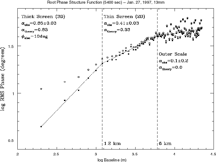
Figure 1 :
The root phase structure function from observations at 13 mm
in the BnA array of the VLA on January 27, 1997 (from Carilli and
Holdaway 1997). The open circles show the rms phase
variations versus baseline length measured on the VLA calibrator
0748+240 over a period of 90 min. The filled squares show these
same values with a constant noise term of 10![]() subtracted in
quadrature. The three regimes of the root phase structure function
as predicted by Kolmogorov turbulence theory are indicated.
subtracted in
quadrature. The three regimes of the root phase structure function
as predicted by Kolmogorov turbulence theory are indicated.
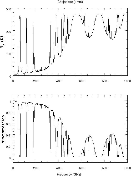
Figure 2: The upper frame shows the radiometric brightness temperature
of the atmosphere for the MMA site at Chajnantor assuming 1 mm of
PWV using the Liebe model (1989). The lower frame shows the corresponding transmission.
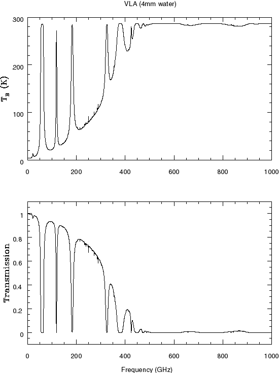
Figure 3: The upper frame shows the radiometric brightness temperature
of the atmosphere for the
VLA site assuming 4 mm of PWV. The lower frame shows the
corresponding transmission.
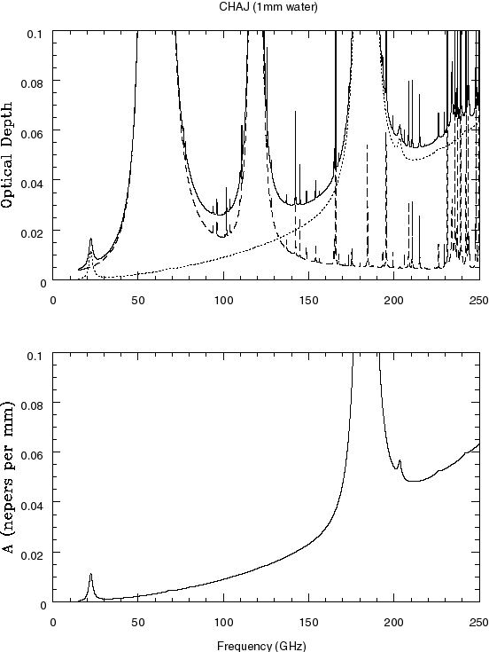
Figure 4: The upper frame shows the optical depth for
MMA site at Chajnantor assuming 1 mm of PWV. The solid line is the
total optical depth. The dotted line is the optical depth due to
PWV. The dash line is the optical depth due to O![]() and other trace
gases. The lower frame shows A
and other trace
gases. The lower frame shows A![]() = optical depth due to 1 mm pf
PWV.
= optical depth due to 1 mm pf
PWV.
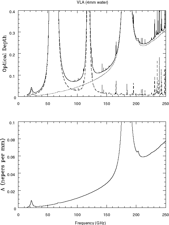
Figure 5: The upper frame shows the optical depth for
VLA site assuming 4 mm of PWV. The solid line is the
total optical depth. The dotted line is the optical depth due to
PWV. The dash line is the optical depth due to O![]() and other trace
gases. The lower frame shows A
and other trace
gases. The lower frame shows A![]() = optical depth due to 1 mm pf
PWV.
= optical depth due to 1 mm pf
PWV.
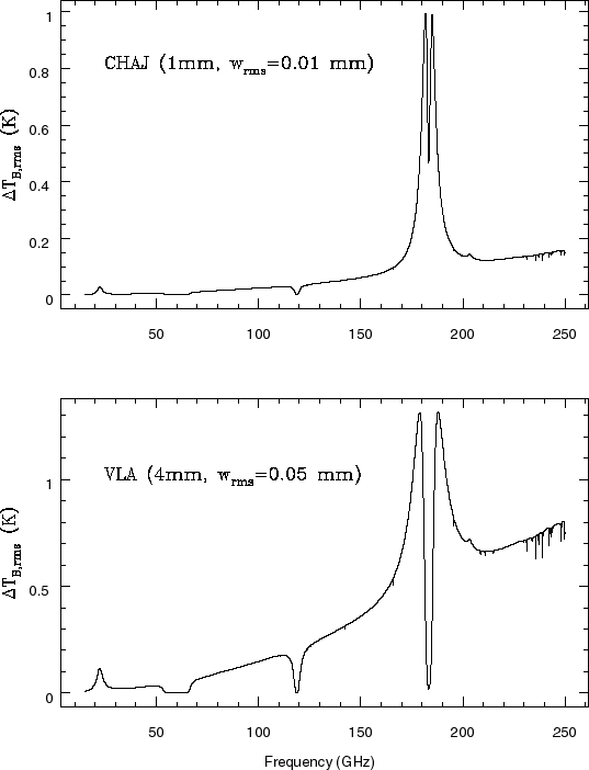
Figure 6: The upper frame shows the expected T![]() for the
MMA site at Chajnantor assuming 1 mm of PWV, and w
for the
MMA site at Chajnantor assuming 1 mm of PWV, and w![]() = 0.01 mm
(equation 5).
The bottom frame shows the expected T
= 0.01 mm
(equation 5).
The bottom frame shows the expected T![]() for the
VLA site assuming 4 mm of PWV, and w
for the
VLA site assuming 4 mm of PWV, and w![]() = 0.05 mm.
= 0.05 mm.
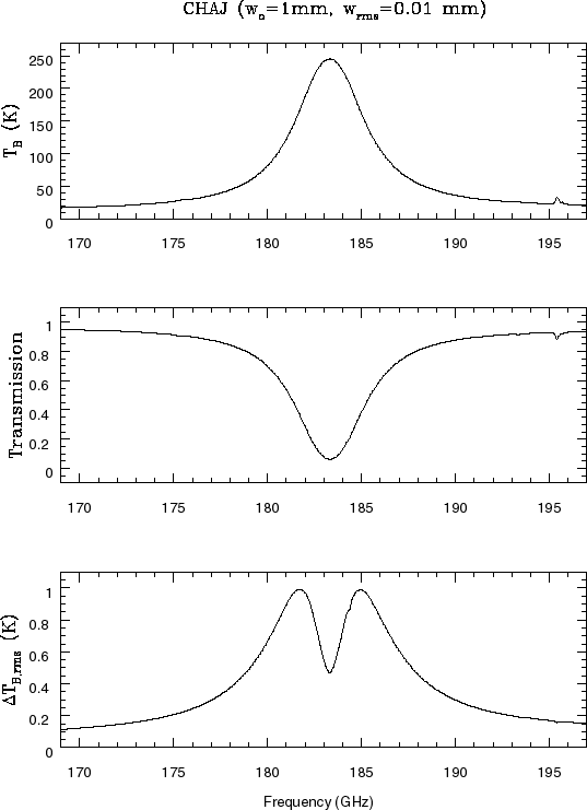
Figure 7: The upper frame shows the expected T![]() for 183 GHz line for
the MMA site at Chajnantor assuming 1 mm of PWV. The middle frame
shows the transmission in this frequency range. The bottom frame shows
the expected T
for 183 GHz line for
the MMA site at Chajnantor assuming 1 mm of PWV. The middle frame
shows the transmission in this frequency range. The bottom frame shows
the expected T![]() assuming w
assuming w![]() = 0.01 mm.
= 0.01 mm.
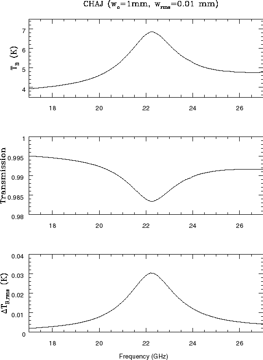
Figure 8: The upper frame shows the expected T![]() for 22 GHz line for
the MMA site at Chajnantor assuming 1 mm of PWV. The middle frame
shows the transmission in this frequency range. The bottom frame shows
the expected T
for 22 GHz line for
the MMA site at Chajnantor assuming 1 mm of PWV. The middle frame
shows the transmission in this frequency range. The bottom frame shows
the expected T![]() assuming w
assuming w![]() = 0.01 mm.
= 0.01 mm.
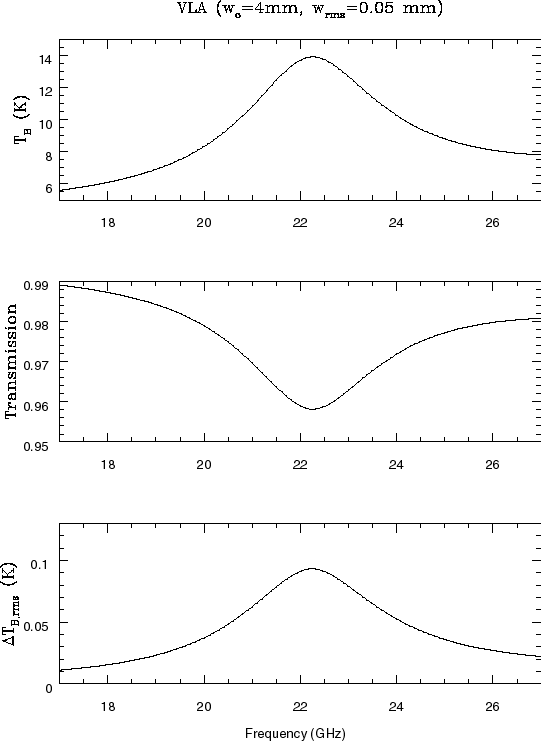
Figure 9: The upper frame shows the expected T![]() for 22 GHz line for
the VLA site assuming 4 mm of PWV. The middle frame
shows the transmission in this frequency range. The bottom frame shows
the expected T
for 22 GHz line for
the VLA site assuming 4 mm of PWV. The middle frame
shows the transmission in this frequency range. The bottom frame shows
the expected T![]() assuming w
assuming w![]() = 0.05 mm.
= 0.05 mm.