I'll present this derivation and some numerical examples in this memo. It turns out that my numbers have a slightly weaker dependence on elevation than Mark's do, e.g., at 20
MMA memo 188:
Another look at anomalous refraction on Chajnantor
Bryan Butler (NRAO)
November 5, 1997
In MMA memo #186 (Holdaway 1997), Mark Holdaway pointed out the
important contribution of atmospheric anomalous refraction to the
pointing error budget for the proposed MMA antennas. He derived
expressions for the magnitude of the effect of anomalous refraction on
the pointing of antennas of different sizes, and calculated values for
proposed MMA antenna sizes for the particular atmospheric
characteristics of the Chajnantor site. I think Mark got the story
right, in that his conclusion was that the pointing error due to
anomalous refraction is smaller in absolute magnitude for larger
antennas, but larger as a fraction of beamwidth. However, it is not
clear that he got the absolute values of the numbers right in the
non-zenith case. He derived a pretty unwieldy equation for the
anomalous refraction for this case (his equation 12), which has some
very non-physical terms in it, and I am not convinced that this
equation is correct. I have derived what I think is the correct
formula for the non-zenith case. This formula is much simpler, and
is (see below for notation):
![]()
I'll present this derivation and some numerical examples in this memo.
It turns out that my numbers have a slightly weaker dependence on
elevation than Mark's do, e.g., at 20![]() my numbers are about 10%
smaller than his (I derive a smaller rms pointing error due to
anomalous refraction). The intent of this memo is not to imply
that Mark did something egregious, but merely to present this simpler
formula, and the new values obtained from it. Again, he got the basic
story right in memo 186.
my numbers are about 10%
smaller than his (I derive a smaller rms pointing error due to
anomalous refraction). The intent of this memo is not to imply
that Mark did something egregious, but merely to present this simpler
formula, and the new values obtained from it. Again, he got the basic
story right in memo 186.
Turbulent fluctuations in the troposphere give rise to differences in
electrical path length across an antenna surface. These differences
can then be thought of as wedges of physical material with an index of
refraction greater than the surrounding air between the points on the
antenna surface. The excess electrical path length (![]() ) and
the physical wedge height (
) and
the physical wedge height (![]() ) are related via:
) are related via:
![]()
where n' is the relative index of refraction of the wedge (the ratio
of the true index of refraction of the wedge to the index of refraction
of the surrounding medium [air]). This is the way that Mark approached
the problem, and I use the same physical model here. These virtual
wedges of material cause plane waves to be redirected as they travel
through, and the net effect over the entire antenna surface is to
produce a pointing error. Another effect is a broadening of the
antenna primary beam. Such effects have been noted for several
antennas on different sites (Altenhoff et al. 1987; Downes & Altenhoff
1990; Church & Hills 1990; Coulman 1991; Zylka et al. 1992; Zylka et al.
1995).
Figure 1 shows a upwardly propagating plane wave incident on a wedge of
length ![]() and height
and height ![]() , both in physical units.
, both in physical units.
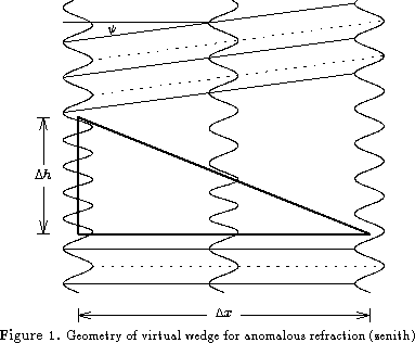
The propagation direction vector of the wave is anti-parallel to the
normal of the wedge lower edge, appropriate for the zenith direction.
Passage through the wedge, which has index of refraction n' relative
to the surrounding medium, causes the wave phase velocity to decrease.
The different thicknesses through the wedge traversed by different
portions of the wave then cause a bending of the wave front, which
is equivalent to a change of direction of the propagation vector of the
wave. The angle between the original propagation direction vector and
the redirected one (![]() ) is the effective pointing error. This
angle can be found by considering the time it takes a wave crest to
cross the distance
) is the effective pointing error. This
angle can be found by considering the time it takes a wave crest to
cross the distance ![]() at the thickest point of the wedge:
at the thickest point of the wedge:
![]()
where ![]() is the phase velocity of the wave in the wedge. This
phase velocity is given by:
is the phase velocity of the wave in the wedge. This
phase velocity is given by:
![]()
with ![]() the phase velocity in the surrounding medium. In time
the phase velocity in the surrounding medium. In time
![]() , the wave crest just beyond the point of the wedge travels a
distance:
, the wave crest just beyond the point of the wedge travels a
distance:
![]()
The angle ![]() is given by:
is given by:
![]()
where ![]() . So,
. So,
![]()
which for small values of ![]() reduces to:
reduces to:
![]()
At any one time, there will be a complicated variation of excess path
length vs position across the projected surface of the antenna. If the
excess path length correlation function is only a function of radial
distance from point to point in the atmosphere, then a 1-D cut through
the 2-D distribution across the projected surface of the antenna is a
good statistical representative of the entire distribution. This 1-D
cut can then be broken up into small intervals (![]() ), each of
which has an effect which is approximated by the wedge treatment
above. The propagation direction vector for the net wave which
emanates from the antenna is then given by a vector sum of each of the
propagation direction vectors for the individual wedges. For each
small wedge, the propagation vector is decomposed into 2 orthogonal
components, one along the direction parallel to the antenna surface
(the x-axis), and the other perpendicular to it (the y-axis).
For an antenna of diameter d, we have
), each of
which has an effect which is approximated by the wedge treatment
above. The propagation direction vector for the net wave which
emanates from the antenna is then given by a vector sum of each of the
propagation direction vectors for the individual wedges. For each
small wedge, the propagation vector is decomposed into 2 orthogonal
components, one along the direction parallel to the antenna surface
(the x-axis), and the other perpendicular to it (the y-axis).
For an antenna of diameter d, we have ![]() small
wedges, and there are values of the excess electrical path length
small
wedges, and there are values of the excess electrical path length
![]() at N + 1 locations. For the
at N + 1 locations. For the ![]() wedge, the two
components of the propagation direction vector are:
wedge, the two
components of the propagation direction vector are:
![]()
and
![]()
![]() is the angle given in equation 8, i.e.,
is the angle given in equation 8, i.e.,
![]() . The propagation
direction vector for the net wave (
. The propagation
direction vector for the net wave (![]() ) is then (for
small
) is then (for
small ![]() ):
):
![]()
If the ![]() are small angles (which they should be), then
are small angles (which they should be), then
![]()
If there are values of the ![]() at M locations (M > N+1),
then the time averaged behavior of the atmosphere flowing over the
antenna can be simulated by virtually sliding the values of the
at M locations (M > N+1),
then the time averaged behavior of the atmosphere flowing over the
antenna can be simulated by virtually sliding the values of the
![]() over the antenna, i.e., there are then M-N+1 values of
the net propagation direction vector, each with pointing error:
over the antenna, i.e., there are then M-N+1 values of
the net propagation direction vector, each with pointing error:
![]()
The rms value of ![]() over the M-N+1 distributions is:
over the M-N+1 distributions is:
![]()
The mean value of the ![]() should be 0 for atmospheric
turbulence, which leaves:
should be 0 for atmospheric
turbulence, which leaves:
![]()
This is directly related to the excess path length structure
function, which is defined as the mean-squared difference of path
length over some distance r (e.g., Tatarski 1961):
![]()
Let r = d, and assume a discrete distribution for ![]() with M-N values at intervals
with M-N values at intervals ![]() , then the discrete
form of the structure function is:
, then the discrete
form of the structure function is:
![]()
which is the form in equation 15. Substituting this in
gives:
![]()
This then is the rms pointing error due to anomalous refraction in an
atmosphere with the specified excess path length structure function,
and is the same as what Mark derives in his equation 9.
The structure function may be written:
![]()
where ![]() and
and ![]() are measured quantities which characterize
the atmosphere for a given location. Given this substitution, the
rms pointing error at zenith for an antenna of diameter d due to
anomalous refraction is given by:
are measured quantities which characterize
the atmosphere for a given location. Given this substitution, the
rms pointing error at zenith for an antenna of diameter d due to
anomalous refraction is given by:
![]()
This means that the absolute value of the anomalous refraction rms
pointing error gets smaller as antenna size gets larger for all
values of ![]() . However, since the width of the primary beam
is proportional to
. However, since the width of the primary beam
is proportional to ![]() , the rms pointing error as a fraction
of primary beam width gets larger as antenna size gets larger
(for
, the rms pointing error as a fraction
of primary beam width gets larger as antenna size gets larger
(for ![]() ). Mark correctly pointed this out.
). Mark correctly pointed this out.
Consider now the case where the same structure of excess path length
exists above the antenna, but it is observed at some angle from the
zenith z. In this case, the time to travel through the thickest
part of the wedge (analagous to equation 3) is given by:
![]()
where the path length through the wedge material is now increased to:
![]()
Proceeding just as in the zenith case gives for the net pointing error:
![]()
where ![]() , reflecting the fact that the
projected size of the antenna on the lower edge of the turbulent layer
is increased by
, reflecting the fact that the
projected size of the antenna on the lower edge of the turbulent layer
is increased by ![]() over its intrinsic size. Again, proceeding as
in the zenith case, the rms pointing error is then:
over its intrinsic size. Again, proceeding as
in the zenith case, the rms pointing error is then:
![]()
This has the same dependence on antenna size as the zenith case, so the
conclusions about the absolute and relative value of the pointing error
vs antenna size in the zenith case also hold here.
The physical basis for the ![]() dependence
on
dependence
on ![]() in equation 24 can be understood as the
combination of two effects. The first is that the physical path length
through the turbulent atmosphere has increased by
in equation 24 can be understood as the
combination of two effects. The first is that the physical path length
through the turbulent atmosphere has increased by ![]() , and hence
the accumulation of excess path length is larger by that same amount.
This means that the amplitude of the structure function is increased by
that amount, and hence the rms increases by
, and hence
the accumulation of excess path length is larger by that same amount.
This means that the amplitude of the structure function is increased by
that amount, and hence the rms increases by ![]() giving rise
to the 1/2 term. The second, as mentioned above, is that the projected
size of the antenna on the lower edge of the turbulent layer is larger
by a factor of
giving rise
to the 1/2 term. The second, as mentioned above, is that the projected
size of the antenna on the lower edge of the turbulent layer is larger
by a factor of ![]() , so the structure function needs to be
evaluated on that larger spatial scale, giving rise to the
, so the structure function needs to be
evaluated on that larger spatial scale, giving rise to the ![]() term. The fact that both of these effects must be
taken into account was noted (and derived) by Taylor (1975). The
increase in the amplitude of the structure function by
term. The fact that both of these effects must be
taken into account was noted (and derived) by Taylor (1975). The
increase in the amplitude of the structure function by ![]() (and
hence an increase in the rms by
(and
hence an increase in the rms by ![]() ) has been noted by many
previous workers (see e.g., Lutomirski & Buser 1974; Tatarski 1961;
Kolchinskii 1957). Kolchinskii (1957) also noted that when different
sets of actual observed variations were fit to a power law in
) has been noted by many
previous workers (see e.g., Lutomirski & Buser 1974; Tatarski 1961;
Kolchinskii 1957). Kolchinskii (1957) also noted that when different
sets of actual observed variations were fit to a power law in ![]() there were many which had a power law exponent > 0.5, which was
unexpected by him. This was most likely the manifestation of the
there were many which had a power law exponent > 0.5, which was
unexpected by him. This was most likely the manifestation of the
![]() term from the argument of the structure function. Note also
that as pointed out by Treuhaft & Lanyi (1987), the
term from the argument of the structure function. Note also
that as pointed out by Treuhaft & Lanyi (1987), the ![]() increase
in the amplitude of the structure function is only valid for baseline
lengths much less than the height of the troposphere (the baseline
length is equivalent to the antenna diameter here). For larger
baseline lengths, the increase is
increase
in the amplitude of the structure function is only valid for baseline
lengths much less than the height of the troposphere (the baseline
length is equivalent to the antenna diameter here). For larger
baseline lengths, the increase is ![]() . This has no bearing on
the problem of anomalous refraction for millimeter antennas, however,
since the antenna diameters are always much smaller than the height of
the troposphere.
. This has no bearing on
the problem of anomalous refraction for millimeter antennas, however,
since the antenna diameters are always much smaller than the height of
the troposphere.
For Chajnantor, the median value of ![]() is 1.2, from Mark's memo.
Using this value, and the values of
is 1.2, from Mark's memo.
Using this value, and the values of ![]() for median
conditions from Table 1 of that memo, the values for the rms pointing
error due to anomalous refraction can then be calculated. These values
are shown in Table 1 for different antenna sizes and different
elevations at Chajnantor. The rms pointing errors relative to the
primary beam size are not shown in Table 1, nor are the values for the
other quartiles of atmospheric conditions. The equivalent values from
Mark's memo are shown in parentheses in Table 1, for comparison. It
seems that my numbers are very slightly smaller than his, as the
dependence on elevation I've derived is somewhat weaker than his.
for median
conditions from Table 1 of that memo, the values for the rms pointing
error due to anomalous refraction can then be calculated. These values
are shown in Table 1 for different antenna sizes and different
elevations at Chajnantor. The rms pointing errors relative to the
primary beam size are not shown in Table 1, nor are the values for the
other quartiles of atmospheric conditions. The equivalent values from
Mark's memo are shown in parentheses in Table 1, for comparison. It
seems that my numbers are very slightly smaller than his, as the
dependence on elevation I've derived is somewhat weaker than his.
Table 1. Anomalous refraction pointing error for median atmospheric conditions at Chajnantor (in arcsec; values in parentheses are from Holdaway [1997]).
ant diam elev angle
(m) 90 ![]()
50 ![]()
30 ![]()
20 ![]()
10 ![]()
8 0.46 (0.47) 0.62 (0.64) 0.99 (1.07) 1.51 (1.65) 3.18 (3.55)
10 0.42 (na) 0.57 (na) 0.91 (na) 1.38 (na) 2.92 (na)
12 0.39 (0.39) 0.53 (0.55) 0.84 (0.90) 1.28 (1.40) 2.70 (3.02)
15 0.36 (0.36) 0.48 (0.49) 0.77 (0.82) 1.17 (1.27) 2.47 (2.76)
50 0.22 (0.22) 0.30 (0.31) 0.48 (0.51) 0.72 (0.79) 1.53 (1.70)
The derivation presented here assumes that geometric optics is
appropriate to describe the propagation of the wave through the
turbulent atmosphere. When the wave optics treatment is included,
the dependence is roughly as I've derived here, but is more complicated
(see e.g., equation 24 of Taylor [1975] [where he uses the Rytov method,
which should be valid for mm-submm wavelengths at Chajnantor] and note
that the pointing error can be directly related to the phase structure
function [or phase correlation function] as easily as to the path
length structure function, i.e., via equation 13.3 of Tatarski
[1961] or equation 73 of Fante [1975]). There is also an implicit
assumption that the turbulence is in a plane parallel slab which is
above the antennas. If the turbulence extends down to the antenna
surface, then the ![]() part of the
part of the ![]() term goes away, since
it is due strictly to the assumed geometry. This plane parallel
assumption will also break down at very low elevations.
term goes away, since
it is due strictly to the assumed geometry. This plane parallel
assumption will also break down at very low elevations.
Altenhoff, W. J., J. W. M. Baars, D. Downes, and J. E. Wink, Observations of anomalous refraction at radio wavelengths, A&A, 184, 381-385, 1987
Church, S., and R. Hills, Measurements of daytime atmospheric ``seeing'' on Mauna Kea made with the James Clerk Maxwell telescope, in Radio Astronomical Seeing, eds. J. E. Baldwin and Wang Shouguan, Pergamon, Oxford, 75-80, 1990
Coulman, C. E., Tropospheric phenomena responsible for anomalous refraction at radio wavelengths, A&A, 251, 743-750, 1991
Downes, D., and W. J. Altenhoff, Anomalous refraction at radio wavelengths, in Radio Astronomical Seeing, eds. J. E. Baldwin and Wang Shouguan, Pergamon, Oxford, 31-40, 1990
Fante, R. L., Electromagnetic beam propagation in turbulent media, Proc. IEEE, 63, 1669-1692, 1975
Holdaway, M., Calculation of anomalous refraction for Chajnantor, MMA memo #186, NRAO, 1997
Kolchinskii, I. G., Some results of observations of the vibration of images of stars at the main astronomical observatory of the academy of sciences of the Ukrainian SSR at Goloseevo, Soviet Astr., 1, 624-636, 1957
Lutomirski, R. F., and R. G. Buser, Phase difference and angle-of-arrival fluctuations in tracking a moving point source, Appl. Opt., 13, 2869-2873, 1974
Tatarski, V. I., Wave Propagation in a Turbulent Medium, Dover, New York, 1961
Taylor, L. S., Effects of layered turbulence on oblique waves, Radio Sci., 10, 121-128, 1975
Treuhaft, R. N., and G. E. Lanyi, The effect of the dynamic wet troposphere on radio interferometric measurements, Radio Sci., 22, 251-265, 1987
Zylka, R., P. G. Mezger, and H. Lesch, Anatomy of the Sagittarius A complex II., A&A, 261, 119-129, 1992
Zylka, R., P. G. Mezger, D. Ward-Thompson, W. J. Duschl, and H. Lesch, Anatomy of the Sagittarius A complex IV., A&A, 297, 83-97, 1995