We present a series of tests of the Fast Switching (FS) phase calibration
technique using the Very Large Array (VLA) at mm wavelengths on
baselines out to 33 km. These tests demonstrate
that FS phase calibration with
cycle times ![]() 100 sec can result in diffraction limited images
of faint sources at 7mm in the largest configurations of the VLA under good
weather conditions. There are times however when shorter cycle times
may be required. We present examples using both `control sources'
(ie. celestial calibrators), and a faint source of astronomical
interest: the M2 supergiant star Betelgeuse (
100 sec can result in diffraction limited images
of faint sources at 7mm in the largest configurations of the VLA under good
weather conditions. There are times however when shorter cycle times
may be required. We present examples using both `control sources'
(ie. celestial calibrators), and a faint source of astronomical
interest: the M2 supergiant star Betelgeuse (![]() Orionis).
A diffraction limited resolution image (40 mas resolution) of the surface
of Betelgeuse was obtained showing a resolved radio photosphere with mean
T
Orionis).
A diffraction limited resolution image (40 mas resolution) of the surface
of Betelgeuse was obtained showing a resolved radio photosphere with mean
T![]() = 3500 K and diameter = 80 mas, consistent with theoretical
models of this star.
= 3500 K and diameter = 80 mas, consistent with theoretical
models of this star.
We also present the tropospheric root phase
structure function on baselines ranging from 200m to 20000m. This
function shows the three regimes predicted by Kolmogorov turbulence theory:
On short baselines (b ![]() 1.2 km) the measured power-law index
is n = 0.85
1.2 km) the measured power-law index
is n = 0.85![]() 0.03, while the predicted value is 0.83
(thick screen). On intermediate
baselines (1.2
0.03, while the predicted value is 0.83
(thick screen). On intermediate
baselines (1.2 ![]() b
b ![]() 6 km)
the measured index is 0.41
6 km)
the measured index is 0.41![]() 0.03 and the predicted value
is 0.33 (thin screen). On long baselines (b
0.03 and the predicted value
is 0.33 (thin screen). On long baselines (b ![]() 6 km) the measured index is
0.1
6 km) the measured index is
0.1![]() 0.2 and the predicted value is zero (outer scale).
The implication is that
the vertical extent of the turbulent boundary layer is about 1 km, and that the
outer scale of the turbulence is 6 km, although the long baseline
data suggests that the outer scale may be anisotropic.
0.2 and the predicted value is zero (outer scale).
The implication is that
the vertical extent of the turbulent boundary layer is about 1 km, and that the
outer scale of the turbulence is 6 km, although the long baseline
data suggests that the outer scale may be anisotropic.
In the forth quarter of 1996 (October 1996 to January 1997) the Very Large Array was in its 33km configuration (`A array'). During this period antennas with 7 mm receivers were situated at the ends of each arm in order to obtain the full resolution of the array for the first time (40 mas). The theoretical sensitivity for the array is 0.1 mJy in 12hrs at 7 mm (13 antennas, 50 MHz bandwidth, 2polarizations, 2IFs), hence the brightness temperature sensitivity is 60 K at 40 mas resolution. These baselines are an order of magnitude longer than for any previous connected-element interferometer operating at mm wavelengths.
One reason for going to the longest baselines with the 7 mm
antennas at the VLA was to test whether
the Fast Switching (FS) phase calibration technique would allow for
diffraction limited
imaging of faint sources on the longest baselines (Carilli, Holdaway,
and Sowinksi 1996, Holdaway and Owen 1995).
Otherwise, the spatial resolution will be limited by tropospheric
`seeing': ![]()
where ![]() = observing wavelength, and
= observing wavelength, and ![]() = the transverse
scale over which the rms phase difference equals one radian
(Narayan et al. 1990). Even under the best conditions at the VLA the limiting
resolution would be about 0.4'' due to tropospheric phase fluctuations.
Fast Switching phase calibration entails standard phase transfer from
a strong celestial calibration source to a faint target source using a
cycle time short enough to `stop' the tropospheric phase fluctuations
at level well below 1 rad. We will show that under typical conditions
at the VLA during the forth quarter of 1996,
the FS technique was adequate to obtain
images of faint sources with diffraction
limited spatial resolution on arbitrarily long baselines at 7 mm.
= the transverse
scale over which the rms phase difference equals one radian
(Narayan et al. 1990). Even under the best conditions at the VLA the limiting
resolution would be about 0.4'' due to tropospheric phase fluctuations.
Fast Switching phase calibration entails standard phase transfer from
a strong celestial calibration source to a faint target source using a
cycle time short enough to `stop' the tropospheric phase fluctuations
at level well below 1 rad. We will show that under typical conditions
at the VLA during the forth quarter of 1996,
the FS technique was adequate to obtain
images of faint sources with diffraction
limited spatial resolution on arbitrarily long baselines at 7 mm.
Phase variations due to the troposphere are caused
by temporal changes in the water vapor content. The implied changes
in index of refraction are
non-dispersive, and hence the phase-variations will increase
linearly with frequency (Tatarskii 1978). The standard model for these
fluctuations is the `frozen screen' approximation, in which variations
in the water vapor column density occur
in a turbulent layer in the troposphere at
some height, H, with some vertical extent, W, which
convects across the array at some velocity, V![]() .
The convection timescale for water vapor irregularities
is assumed to be shorter than the
dissipation (or diffusion) timescale and hence the phase screen is
`frozen-in' to the flow (Taylor 1938, Wright
1996). Under this assumption one can relate temporal and spatial
phase fluctuations using V
.
The convection timescale for water vapor irregularities
is assumed to be shorter than the
dissipation (or diffusion) timescale and hence the phase screen is
`frozen-in' to the flow (Taylor 1938, Wright
1996). Under this assumption one can relate temporal and spatial
phase fluctuations using V![]() .
.
Tropospheric phase fluctuations are usually
characterized by a root phase structure function,
![]() (b), equal to the root mean square phase variations on
baselines of length b, when calculated over a sufficiently long time
(time >> baseline crossing time =
(b), equal to the root mean square phase variations on
baselines of length b, when calculated over a sufficiently long time
(time >> baseline crossing time = ![]() ),
or for an ensemble of measurements at a given
time on many baselines of length b. Kolmogorov
turbulence theory (Coulman 1990) predicts a function of the form:
),
or for an ensemble of measurements at a given
time on many baselines of length b. Kolmogorov
turbulence theory (Coulman 1990) predicts a function of the form:
![]()
where b is in km, and ![]() is in cm. Typical values of K for the
VLA can be found in Carilli etal. (1996).
is in cm. Typical values of K for the
VLA can be found in Carilli etal. (1996).
Kolmogorov turbulence theory predicts
n = ![]() for baselines longer than W,
and n =
for baselines longer than W,
and n = ![]() for baselines
shorter than W (Coulman 1990). The change in power-law index at b = W is
due to the finite vertical extent
of the turbulent boundary layer. For baselines
shorter than the typical turbulent layer extent the full 3-dimensionality
of the turbulence is involved (thick-screen), while for longer baselines
a 2-dimensional approximation applies (thin-screen).
Turbulence theory also predicts an `outer-scale', L
for baselines
shorter than W (Coulman 1990). The change in power-law index at b = W is
due to the finite vertical extent
of the turbulent boundary layer. For baselines
shorter than the typical turbulent layer extent the full 3-dimensionality
of the turbulence is involved (thick-screen), while for longer baselines
a 2-dimensional approximation applies (thin-screen).
Turbulence theory also predicts an `outer-scale', L![]() , beyond which the
structure function should be flat (n = 0). This scale corresponds to
the largest coherent structures, or maximum correlation length,
for water vapor fluctuations in the troposphere, presumably set by
external boundary conditions.
, beyond which the
structure function should be flat (n = 0). This scale corresponds to
the largest coherent structures, or maximum correlation length,
for water vapor fluctuations in the troposphere, presumably set by
external boundary conditions.
Measurements of the root phase structure function have
been made on baselines out to 3 km (Sramek 1990, Holdaway et al. 1995,
Holdaway and Owen 1995, Wright 1996, Carilli etal. 1996).
These measurements have demonstrated the basic broken
power-law behavior (n = 5/6 to n = 1/3), with the transition occuring
at about 1 km, although power-laws of intermediate indices have also
been seen (Holdaway and Owen 1995, Holdaway etal. 1995).
However, to date no measurement has been made of the
full structure funtion, from b << W to b >> L![]() .
The difficulty is that the outer scale is
predicted to be of order 10 km (Coulman 1990),
thereby requiring the A configuration of
the VLA. However, the shortest baselines in the A configuration are
about 1 km, hence observations with the A array alone do not sample b
< W.
.
The difficulty is that the outer scale is
predicted to be of order 10 km (Coulman 1990),
thereby requiring the A configuration of
the VLA. However, the shortest baselines in the A configuration are
about 1 km, hence observations with the A array alone do not sample b
< W.
As part of our testing with the VLA we performed a
measurement of the root phase structure function using the mixed BnA
configuration. This configuration has good baseline coverage ranging
from 200m to 20 km, hence sampling all three ranges in the structure
function. The resulting root phase structure function is shown in
Figure 1,
for 13 mm observations made during the night of Jan. 27, 1997 on
the VLA calibration source 0748+240. The total observing time was 90
min, corresponding to a tropospheric travel distance of 54 km, assuming
V![]() = 10 m s
= 10 m s![]() (see below).
Below we shall find that 54 km is much larger than the
outer scale of the turbulence, hence
90 minutes corresponds to many realizations of the
phase screen at b = L
(see below).
Below we shall find that 54 km is much larger than the
outer scale of the turbulence, hence
90 minutes corresponds to many realizations of the
phase screen at b = L![]() .
.
The open circles show the nominal tropospheric root phase structure
function = rms phases for the visibilities versus baseline length
calculated over the full 90 min time range. The
solid squares are the rms phases after subtracting (in
quadrature) a constant electronic noise term of 10![]() , as derived from
the data by requiring the best power-law on short baselines.
The 10
, as derived from
the data by requiring the best power-law on short baselines.
The 10![]() noise term is consistent with previous measurements at the
VLA indicating electronic phase noise increasing with frequency as
0.5
noise term is consistent with previous measurements at the
VLA indicating electronic phase noise increasing with frequency as
0.5![]() per GHz (Carilli and Holdaway 1996).
per GHz (Carilli and Holdaway 1996).
The three regimes of the structure function as predicted
by theory are verified very nicely
in
Figure 1,
and the observed power-law indices
are in good agreement with the predicted values.
On short baselines (b ![]() W = 1.2 km) the measured index
n = 0.85
W = 1.2 km) the measured index
n = 0.85![]() 0.03, while the predicted value is 0.83. On intermediate
baselines (W
0.03, while the predicted value is 0.83. On intermediate
baselines (W ![]() b
b ![]() L
L![]() = 6 km)
the measured index is 0.41
= 6 km)
the measured index is 0.41![]() 0.03 and the predicted value
is 0.33. On long baselines (b
0.03 and the predicted value
is 0.33. On long baselines (b ![]() L
L![]() = 6 km) the measured index is
0.1
= 6 km) the measured index is
0.1![]() 0.2 and the predicted value is zero. The implication is that
the vertical extent of the turbulent boundary layer is about 1 km, and that the
outer scale of the turbulence is 6 km.2
0.2 and the predicted value is zero. The implication is that
the vertical extent of the turbulent boundary layer is about 1 km, and that the
outer scale of the turbulence is 6 km.2
Another trend that is clear in Figure 1
is that the scatter increases
significantly beyond the outer scale. A possible explanation for this
increased scatter is shown in Figure 2.
The open circles in Figure 2
are rms phases for baselines
between antennas on the north arm and the south-west arm of the
array. The filled squares are rms phases for baselines
between antennas on the north arm and the south-east arm of the
array. The two functions are similar (to within the noise)
out to about 6 km. Beyond 6 km the open circles continue to rise, while
the filled squares flatten to zero slope.
This trend may indicate an anisotropic outer scale, such that the
structure function `saturates' at different baseline lengths depending
on the orientation of the baseline. An anisotropic outer scale could
arise e.g., due to anisotropic boundary conditions.
For completeness we note that the
ground wind speed during these observations was 2 m s![]() from the
southeast, ie. parallel to the southeast arm. It is important
to keep in mind that the ground wind speed may bear little relation to
the more relevant speed of the winds aloft.
from the
southeast, ie. parallel to the southeast arm. It is important
to keep in mind that the ground wind speed may bear little relation to
the more relevant speed of the winds aloft.
As a demonstration of the effectiveness of fast switching phase calibration, we have calculated the root phase SF for the BnA array data at 13 mm after applying antenna-based phase solutions averaged over increasingly shorter timescales. The results are shown in Figure 2. The solid squares show the nominal tropospheric root phase SF from Figure 1, but now on a linear scale. The open circles are the rms phases of the visibilities after applying antenna based phase solutions averaged over 300 sec. The stars are the rms phases of the visibilities after applying antenna based phase solutions averaged over 20 sec.
The residual root SF using a 300 sec calibration cycle
parallels the nominal tropospheric root SF out to a baseline length of
1500m, beyond which the root SF saturates at a constant rms phase value of
20![]() . Calibrating with relatively short cycle times
`stops' the tropospheric phase variations at an effective baseline
length: b
. Calibrating with relatively short cycle times
`stops' the tropospheric phase variations at an effective baseline
length: b![]() =
= ![]() (Carilli et al. 1996).
The implied wind velocity is then: V
(Carilli et al. 1996).
The implied wind velocity is then: V![]() =
= ![]() = 10 m s
= 10 m s![]() . Going to a 20 sec calibration
cycle reduces b
. Going to a 20 sec calibration
cycle reduces b![]() to only 100 m, which is shorter than the shortest
baseline of the array, and the saturation rms is 5
to only 100 m, which is shorter than the shortest
baseline of the array, and the saturation rms is 5![]() .
.
The important point is that, after applying standard phase calibration
techniques on timescales short compared to the tropospheric crossing,
the resulting rms phase fluctuations are independent of baseline
length for b > b![]() .
.
Fast Switching phase calibration was employed extensively at 7 mm
during the forth quarter of 1997. We present one example in which
FS calibration was effective in allowing for diffraction limited
imaging of a faint celestial target source. The target source was the
M2 supergiant star Betelgeuse (![]() Orionis). The optical photospheric
diameter for the star is 65 mas (Tuthill et al. 1997), while the
integrated flux density of the star is 27 mJy at 7 mm. Hence the
star is large enough to be resolved by the VLA at 40 mas resolution,
and bright enough to be detected, but not bright enough to allow for
self-calibration on short timescales. Diffraction limited imaging
of the star requires the FS phase transfer technique.
Orionis). The optical photospheric
diameter for the star is 65 mas (Tuthill et al. 1997), while the
integrated flux density of the star is 27 mJy at 7 mm. Hence the
star is large enough to be resolved by the VLA at 40 mas resolution,
and bright enough to be detected, but not bright enough to allow for
self-calibration on short timescales. Diffraction limited imaging
of the star requires the FS phase transfer technique.
The Betelgeuse observations were made
over the night of December 21, 1996.
We used the celestial calibrator 0552+032
located 4![]() degrees from the target source, with a total cycle time
of 150 sec. Figure 4
shows the time series of antenna-based phase
solutions on the calibrator
for these observations for three antennas on the north arm of
the VLA. The total observing time was 10hrs. The phase stability was
excellent between IAT 3:00 and 9:00. After 9:00 the phase stability
deteriorated signficantly. Figure 5
shows images of Betelgeuse made by
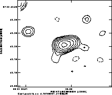
applying the FS phase calibration solutions from 0552+032. Figure 5A
shows the image made from data taken during the time when the phase
stability was good (3 - 9 IAT), while Figure 5B shows the image made from
data taken during the time when the phase stability deteriorated (9 - 12
IAT). The image from the good time period reveals a resolved, possibly
asymmeteric source, with a diameter of about 80 mas and an average brightness
temperature of 3500 K, as expected for the radio photosphere of this M2
supergiant (Lim et al. 1997).
The image from the bad time range reveals a source, but
the structure and brightness are uncertain due to the poor phase
stability. In other words, the 150 sec cycle was adequate to
obtain reasonable phase transfer from the calibrator to the source
during good weather, but was inadequate when the weather
deteriorated. It is likely that a faster cycle time might have been
able to recover a reasonable image of the source even during the bad
time period.
The observing log reports an increase in the ground wind speed from
2.9 m s
degrees from the target source, with a total cycle time
of 150 sec. Figure 4
shows the time series of antenna-based phase
solutions on the calibrator
for these observations for three antennas on the north arm of
the VLA. The total observing time was 10hrs. The phase stability was
excellent between IAT 3:00 and 9:00. After 9:00 the phase stability
deteriorated signficantly. Figure 5
shows images of Betelgeuse made by
applying the FS phase calibration solutions from 0552+032. Figure 5A
shows the image made from data taken during the time when the phase
stability was good (3 - 9 IAT), while Figure 5B shows the image made from
data taken during the time when the phase stability deteriorated (9 - 12
IAT). The image from the good time period reveals a resolved, possibly
asymmeteric source, with a diameter of about 80 mas and an average brightness
temperature of 3500 K, as expected for the radio photosphere of this M2
supergiant (Lim et al. 1997).
The image from the bad time range reveals a source, but
the structure and brightness are uncertain due to the poor phase
stability. In other words, the 150 sec cycle was adequate to
obtain reasonable phase transfer from the calibrator to the source
during good weather, but was inadequate when the weather
deteriorated. It is likely that a faster cycle time might have been
able to recover a reasonable image of the source even during the bad
time period.
The observing log reports an increase in the ground wind speed from
2.9 m s![]() to 5.5 m s
to 5.5 m s![]() , and an increase in stratusform-type
cloud cover from 50
, and an increase in stratusform-type
cloud cover from 50![]() to 100
to 100![]() , during the time period when the
phase stability deteriorated.
, during the time period when the
phase stability deteriorated.
In Figure 6
we show the root phase structure functions for the
periods of good and bad weather for the December 21 observaitons.
Also shown are the residual root SFs
after self-calibration with a 35 sec averaging time.
Two trends are apparent. The first is
that during the bad time period the steep part of the structure
function continues to longer baselines (> 10 km).
The second is that the residual saturation RMS
(after self-calibration) increases from 8![]() during the good time
period to 14
during the good time
period to 14![]() during the bad time period.
The possible implications are that: (i) the turbulent region in the
troposphere became thicker during the bad time period, and (ii) the
amplitude in the structure function (the `K' value) increased, from
about 24 during the good time period, to 42 during the bad time period.
during the bad time period.
The possible implications are that: (i) the turbulent region in the
troposphere became thicker during the bad time period, and (ii) the
amplitude in the structure function (the `K' value) increased, from
about 24 during the good time period, to 42 during the bad time period.
As an independent check on possible extraneous structure
introduce by residual tropospheric phase variations after FS phase
calibration, we used two 15min time periods during the December
observations to switch between the calibrator 0552+032 and a `control
source,' namely the celestial calibrator 0532+075,
with the same cycle time as was
employed on Betelgeuse. The results are shown in
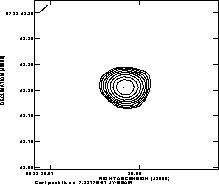
Figure 7. Figure 7A
shows the image of the control source 0532+075 made after
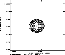
self-calibration with an averaging time of 10sec (the nominal `true' image).
Figure 7B shows the image of 0532+075 made by transfering phase
solutions from the 0552+032 with an averaging time of 900 sec.
Figure 7C shows the image of 0532+075
made by transfering phase
solutions from the 0552+032 with a cycle time of
150sec. The 900 sec cycle time results in an
extended image, while the 150 sec cycle time shows a
point source with some minor structure due to residual
phase errors. The image coherence increases from
42![]() with a 900 sec calibration cycle time to 72
with a 900 sec calibration cycle time to 72![]() with a 150 sec
cycle time, where the coherence is defined as the ratio of the peak
surface brightness on the phase-referenced image
relative to that seen on the self-calibrated image.
with a 150 sec
cycle time, where the coherence is defined as the ratio of the peak
surface brightness on the phase-referenced image
relative to that seen on the self-calibrated image.
We have demonstrated that the FS phase calibration technique with
cycle times ![]() 100 sec can result in diffraction limited images
of faint sources in the largest configurations of the VLA under good
weather conditions. There are times however when shorter cycle times
may be required. The NRAO has installed at the VLA site
a two element interferometer
tracking a satellite beacon at 11.3 GHz to act as a
monitor of the tropospheric phase stability (Radford et al. 1996).
Data from this monitor
should help observers in making real-time decisions concerning required
calibration cycle times for high frequency observations with the VLA,
as well as provide a quantitative seasonal and diurnal record of the
phase stability of the VLA site, in order to facilitate efficient
scheduling of observing programs that are sensitive to tropospheric
phase fluctuations.
100 sec can result in diffraction limited images
of faint sources in the largest configurations of the VLA under good
weather conditions. There are times however when shorter cycle times
may be required. The NRAO has installed at the VLA site
a two element interferometer
tracking a satellite beacon at 11.3 GHz to act as a
monitor of the tropospheric phase stability (Radford et al. 1996).
Data from this monitor
should help observers in making real-time decisions concerning required
calibration cycle times for high frequency observations with the VLA,
as well as provide a quantitative seasonal and diurnal record of the
phase stability of the VLA site, in order to facilitate efficient
scheduling of observing programs that are sensitive to tropospheric
phase fluctuations.
Carilli, C.L., Holdaway, M.A., and Sowinski, K. 1996,VLA Scientific Memo. No. 169
Carilli, C.L. and Holdaway, M.A. 1996,VLA Scientific Memo. No. 171
Coulman, C.E. 1990, in Radio Astronomical Seeing, eds. J. Baldwin and S. Wang, (Pergamon: New York), p. 11.
Holdaway, M.A., Radford, S., Owen, F., and Foster, S. 1995, MMA Memo. Series.
Holdaway, M.A. and Owen, F.N. 1995, MMA Memo. No. 126
Holdaway, M.A. Owen, F., and Rupen, M.P. 1994, MMA Memo. No. 123
Holdaway, M.A. 1992, MMA Memo. No. 84
Lim, J., Carilli, C.L., White, S., Beasley, A., and Marson, R. 1997, in preparation
Narayan, R., Anatharamiah, K., and Cornwell, T. 1990, in Radio Astronomical Seeing, eds. J. Baldwin and S. Wang, (Pergamon: New York), p. 205
Radford, S.J., Reiland, G., and Shillue, B. 1996, P.A.S.P., 108, 441
Sramek, R. 1990, in Radio Astronomical Seeing, eds. J. Baldwin and S. Wang, (Pergamon: New York), p. 21
Tatarskii, V.I. 1961, Wave Propagation in Turbulent Media, (New York: Wiley)
Taylor, G.I. 1938, Proc. R. Soc. London A, 164, 476
Tuthill, P.G., Haiff, C.A., and Baldwin, J.E. 1997, M.N.R.A.S., 285, 529
Wright, M.C.H. 1996, P.A.S.P., 108, 520
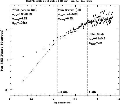
Figure 1: The root phase structure function from observations at 13 mm
in the BnA array of the VLA on January 27, 1997.
The open circles show the rms phase
variations versus baseline length measured on the VLA calibrator
0748+240 over a period of 90 min. The filled squares show these
same values with a constant noise term of 10![]() subtracted in
quadrature.
subtracted in
quadrature.
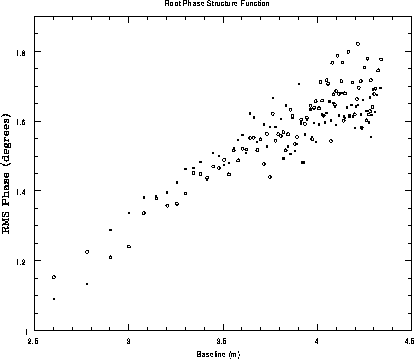
Figure 2: Same as Figure 1, but now the open cicles are the
root phase structure function for baselines between antennas
on the north arm of the array
with those on the southwest arm, while the filled squares
are for baselines between antennas on the north arm with those on the
southeast arm.
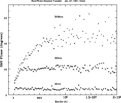
Figure 3: The solid squares are the same as for Figure 1, but now
on a linear scale. The open cicles show the residual rms phase
variations versus baseline length
after calibrating with a cycle time of 300sec.
The open stars show the residual rms phase
variations versus baseline length
after calibrating with a cycle time of 20sec.
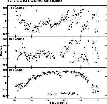
Figure 4: The time series of antenna-based phase solutions on the
calibrator 0552+032 for three antennas on the north arm at 7 mm
on December 21, 1996.
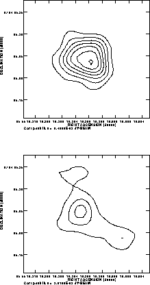
Figure 5: The top figure shows an image of the star Betelgeuse at
7 mm, 40mas resolution made from data taken during the time period
of good phase stability (3 - 9 IAT) the night of Dec. 21,
1997. The lower image shows the image of Betelgeuse made from data
taken during the time period of bad phase stability (9 - 12 IAT)
IAT). The contour levels are
-1.8, -0.9, 0.9, 1.8, 2.7, 3.6, 4.5, 5.4, and 6.3 mJy/beam.
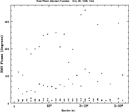
Figure 6: The rms phase variations versus baseline length
measured on the calibrator
0552+032 on Dec. 21, 1997 at 7 mm with the VLA.
The stars are the rms phases from the bad phase stability time
period (9 - 12 IAT). The solid squares are the rms phases from the good time
period (3 - 9 IAT). The open circles are the residual
rms phases from the bad time period after applying phase calibration
with a 35 sec averaging time. The open stars are the residual rms phases
from the good time period after applying phase calibration
with a 35 sec averaging time.