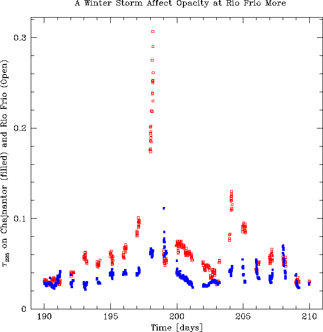
Figure: 1 Opacity time series for the two sites. Filled squares are Chajnantor, open squares are Rio Frio, time is in days since 0 hours UT, Jan 1, 1995. This plot only includes data when the radiometers at both sites were functional.
MMA Memo 152: Comparison of Rio Frio and Chajnantor Site Testing Data
K. Kohno, F.N. Owen, S.J.E. Radford, M. Saito
April 19, 1996
We investigate the site testing data from the Rio Frio and Chajnantor sites in northern Chile over the period July 1995 through February 1996. The 225 GHz opacities are about 40% higher at Rio Frio than at Chajnantor, smaller than the 65% which would be expected if the difference in opacities were due entirely to the 1000 m difference in elevation (assuming a 2 km scale height). The rms phase fluctuations are about 20% higher at Rio Frio than at Chajnantor. Neither site shows very much diurnal variation in opacity. Both sites show very similar diurnal variations of rms phase, phase structure function exponent, and the speed of the turbulent water vapor above the site. Most differences between the two sites in these diurnal variations can be explained in terms of the difference in elevation.
The effects of the ``Bolivian Winter'', a southern hemisphere summer weather trend in which the winds come out of the east, bringing moisture from the Amazon basin to Chile, do not affect the quality of the Chajnantor site much more than the quality of the Rio Frio site. It was initially thought that the proximity of the Chajnantor site to the source of the Bolivian Winter's moisture might adversely affect the phase stability and opacity at the Chajnantor site relative to the Rio Frio site. During the very worst phase and opacity conditions, Chajnantor does perform slightly worse than Rio Frio, but the improved performance at Chajnantor during the good times greatly outweighs this trend.
NRO began operation of two weather stations, a 220 GHz tipping radiometer, and a 11.2 GHz, 300 m radio seeing monitor at the 4050 m Rio Frio site in northern Chile in early July, 1995. NRAO began operation of an identical weather station, a 225 GHz radiometer, and an almost identical radio seeing monitor around April 1995 at the 5050 m Chajnantor site (also called the San Pedro site) about 300 km distant from the Rio Frio site. This work makes a preliminary comparison of the opacity and phase stability data from these two sites.
That the two radiometers operate at different frequencies is not unimportant. Earlier side by side comparisons made at Paranal indicated the instruments were measuring the same opacity to within about 0.01. However, atmospheric models indicate the opacity at the two different frequencies should be more different than what was observed. At 5000 m, Liebe's model predicts that
where is the precipitable water vapor in millimeters. When we consider that the 4000 m site will experience more pressure broadening in the lines, the opacity at Rio Frio should actually follow something more like One use of the radiometer data is to determine what the opacity is at (or very near) the measured frequency. Since the opacity at 225 GHz should be greater than the opacity at 220 GHz, the Rio Frio opacities should actually be scaled up slightly for comparison with the Chajnantor opacities. Another use of the radiometer data is to estimate the opacity in the submillimeter, which requires the use of models which are possibly in error by as much as 50%. Since the submillimeter opacities are dominated by the PWV, we would need to extract the PWV term from the opacities. At this stage in the site comparisons, we will ignore these details and report only on the measured opacities, remembering that the Rio Frio opacities may need to be shifted to slightly larger values in either a 225 GHz or submillimeter comparison.
Both the Rio Frio and the Chajnantor radiometers have had problems. When a problem occurs and an instrument is down, it is usually several weeks before a trip can be arranged to service the instrument. Furthermore, the Chajnantor radiometer does not perform any opacity measurements for 1 hour out of every 4.5 hours. Hence, out of the eight months for which we have radiometer data from both sites, there is a total of only 24 days time for which both instruments were operating, or about 10% of the possible time. Because the daily and seasonal variations are important, and each instruments' downtime is not randomly distributed in time, a comparison of the two sites' opacity requires that we analize data only when both instruments are running. The instrument on Chajnantor samples the opacity every 10 minutes, while the Rio Frio instrument samples the opacity about once a minute. We have selected the Rio Frio opacity which is closest in time to each measured Chajnantor opacity, to a maximum time offset of 10 minutes, so the resulting database has the same number of opacity measurements for each site, and the measurements sample the seasonal and diurnal variations in the same way.
Figures 1 and 2 show typical time series spanning a couple of weeks for the opacities of each site (in this document, open squares will represent Rio Frio data and filled squares will represent Chajnantor data). Figure 3 shows a scatter plot of Rio Frio opacity against Chajnantor opacity for all available data. There are clearly many times when the opacity is excellent on Chajnantor and less good at the Rio Frio site. Figure 4 shows the cumulative distributions of opacity at the two sites. Table 1 shows the quartile opacities on each site, along with their ratio and the scale height which is implied if the only intrinsic difference between the two sites is elevation. In reality, the two sites do have other differences: the very worst opacities on Chajnantor, associated with the Bolivian winter from the east and some winter storms from the west, are somewhat worse than the worst opacities on Rio Frio. The calculated scale heights of 2.5 km and 3.1 km are similar to the assumed scale height of about 2.0 km. If the only difference between the two sites was the elevation, a 2 km water vapor scale height would result in Rio Frio's opacities being 65% higher than Chajnantor's. We see a marked trend towards larger scale heights as the opacity conditions worsen. This indicates that during the very best conditions, the main difference between the two sites is the elevation, and during worse conditions, other geographical differences, such as Chajnantor's proximity to the Amazon basin, begin to degrade Chajnantor's performance relative to Rio Frio's.
| Quarter | Rio Frio | Chajnantor | Ratio | Scale Height [km] |
| Q1 | 0.045 | 0.0302 | 1.49 | 2.5 |
| Q2 | 0.061 | 0.0443 | 1.38 | 3.1 |
| Q3 | 0.094 | 0.0809 | 1.16 | 6.7 |
Unfortunately, there is not enough data in the combined data set to see any clear diurnal variations. For comparison with the diurnal phase fluctuations below, we therefore include a plot of diurnal opacity variations generated from the full Rio Frio opacity database in Figure 5. Similar to Chajnantor, the diurnal variations in opacity are very small and manifest themselves most in the worst data.
The radio seeing monitors (or site test interferometers) at the two sites are very similar. Both observe an 11.2 GHz beacon from the Intelsat 601 geosynchronous satellite at about 27.5 degrees W longitude and 36 degrees elevation. Both interferometers have 1.8 m antennas on the ends of 300 m E-W baselines. The front ends have very similar noise temperatures (see the thermal noise analysis below), the transmission cables are burried underground to increase the thermal insulation, and all cables above ground are heavily insulated. The Rio Frio instrument correlates the signals with a vector voltmeter, while the Chajnantor instrument performs a digital correlation with the PC which controls and monitors the instrument and its incoming data.
The data reduction path which we use was pionered by Holdaway, Ishiguro, and Morita (1996, in preparation), and refined in Holdaway et al (1995), in which the data reduction for the May 1995 Chajnantor site test interferometer data was discussed. We discuss here some of the details of the Rio Frio data reduction.
The gross motion of the satellite in the sky is much smaller than the primary beam of the 1.8 m dishes, but sufficient to cause many turns of phase per day. Since the atmospheric phase fluctuations we want to characterize are about 1 degree rms, we must remove the bulk phase caused by the satellite motion. Furthermore, the phase drift caused by the satellite motion often changes from day to day due to changes in the satellite's orbital parameters. We learned from the Chajnantor data that we required a 600 s (many crossing times of the 300 m baseline) time series of phase data to solve for the phase structure1 function power law exponent and the velocity of the turbulent water vapor. Removing a second order polynomial trend from the raw phases on 600 s time scales was sufficient to remove the effects of satellite motion (and probably some thermal drifts as well), but usually results in under 1% reduction of the true atmospheric phase noise (as determined by atmospheric simulations with typical structure function exponents and wind velocities of 5 m/s or greater).
When we investigated the Rio Frio time series, we found some anomalous phase excursions. Figure 6 shows the raw phase data for both the Rio Frio and Chajnantor instruments for December 10, 1995. The similarity in the trends of the bulk phase indicate that both instruments are very likely observing the same satellite. However, the Rio Frio phase contains a number of bumps and excursions from the bulk phase trend. These excursions are generally on time scales of 10-60 minutes, and are apparent about 5-10% of the time on about 75% of the days. Since we are looking at 10 minute time series for the phase analysis, the shorter time scale anomalous excursions are leeking into our results at some level, biasing them towards larger rms path length variations, and perhaps steeper structure function power law exponents and lower velocities of the turbulent water vapor. The 20 minute phase time series shown in Figure 7 shows an expanded view of a phase blip similar to the smaller ones in the day-long plot in Figure 6. While a second order polynomial trend would remove most of the problem for 10 minute time series in this example, some residual problems would persist. Furthermore, similar incidents of slightly shorter time scale would not be addressed at all by removing a second order polynomial trend.
We find that these anomalous phase excursions are not correlated with time of day, the measured weather data (temperature, wind velocity, wind direction, water vapor pressure, and solar flux) or their time derivatives. We conclude that they are due to electronic instabilities in the Rio Frio radio seeing monitor. In order to reduce the effect of these phase excursions on the data, we could remove a third order polynomial fit to the bulk phase over each 600 s phase time series to try to counteract the effect of the anomalous long time scale phase excursions. A test on Chajnantor data, which did not suffer from this problem, indicated that the median phase was decreased by 7% when removing a third order polynomial trend rather than a second order trend; presumably the decrease was due mainly to removing atmospheric phase noise, rather than instrumental instabilities. When we reduced the Rio Frio data with both the second order polynomial and the third order polynomial trends removed, we found that the median rms phase was only 10% lower for the third order polynomial trend. Since this is similar to the Chajnantor case, we conclude that the effect of the anomalous phase excursions on the results is on the order of a few percent after the 2nd order polynomial trend is removed. When comparing the Rio Frio and Chajnantor data, we should remember that the Rio Frio data may be slightly biased in this way.
The Chajnantor site testing interferometer initially had a 1 s thermal noise level of 0.16 degrees (calculated empirically from the shortest time scales of the temporal phase structure functions), but equipping the front ends with circular polarizers in the same sense of the satellite radiation has reduced the noise level by to 0.11 degrees. We have identified a similar white noise term of 0.18 degrees in the Rio Frio instrument (leading to a noise of 0.18* = 0.25 in the structure function, which is calculating by differencing the interferometer phases at different times). Figure 8 indicates a typical phase structure function for good seeing conditions. The open boxes represent the calculated structure function, which is affected by noise on the short time scales, and the filled boxes, which lie right on the best fit line, represent the structure function after quadratically correcting for the 0.25 degree noise term. The 0.18 degree noise adds quadratically with the rms phase over 600 s, and is usually only a minor contribution as the atmospheric phase fluctuations are usually above 1 degree rms, with the minimum being about 0.3 degrees rms. However, the 0.25 degree noise term in the structure function often has a major effect on the structure function's power law exponent: before correcting for the noise, the structure function shown in Figure 8 had a power law exponent of 0.34, and after correction the exponent became 0.62.
In this section, we derive a few results using all of the available phase data from Rio Frio, but we make no comparisons with the Chajnantor based on these results.
Of primary interest is the diurnal variation of the rms phase. On both Mauna Kea and Chajnantor, the diurnal phase variations are found to be much larger than the diurnal opacity variations. We confirm that trend for Rio Frio. Figure 9 shows the best rms phases and the first, second, and third quartiles as a function of local hour of the day. The day time fluctuations are typically three times larger than the night time fluctuations. Compare this with the almost nonexistent diurnal opacity fluctuations in Figure 5. The apparent dip in the rms phase near midday is actually an artifact of the time which was sampled by the Rio Frio radio seeing monitor: during much of December and January, data was taken only from midnight until noon. Since this was local summer, the season of poorest phase stability, the quartiles in the first twelve hours of the day, and especially between 8am and noon, were boosted up by the inclusion of this data. So, the midday dip is actually a lack of boosting up due to missing summertime data during these hours.
Kolmogorov turbulence in an atmospheric layer which is much thinner than the interferometer baseline length results in a structure function exponent of 0.33, while thick turbulence results in an exponent of 0.83. Intermediate slopes can be obtained by a linear combination of thin and thick layers. Prior to removing the white noise term, the structure function exponent on Rio Frio was often between 0.1 and 0.3 during the good phase conditions which are most affected by the white noise. A histogram of the structure function exponents after the white noise correction is shown in Figure 10. Reassuringly, only a small fraction of the data results in structure function exponents outside the theoretical range. The shape of the histogram is qualitatively similar to that of the Chajnantor site.
In Figure 11, we show the variation of the structure function exponent with time of day. The most interesting trend here is the flattening of the exponent which occurs at midday. Most sites (Nobeyama, Mauna Kea, and Chajnantor) display a marked flattening of the structure function exponent as the rms phase fluctuations decrease. Rio Frio shows the same general trend, but there are many times when the rms phase is high and the exponent is low, and many times when the rms phase is low but the exponent is high.
Our analysis of the radio seeing monitor data allows us to determine the velocity of the turbulent water vapor over the interferometer. A diurnal plot of the lowest ``wind aloft'' speed and the first, second, and third quartile values is shown in Figure 12. The winds aloft show a weak diurnal variation, actually decreasing during the daytime. Contrast this to the surface winds, which show a strong diurnal variation and get much faster during the daytime. However, the slower daytime winds aloft are still faster than the fast daytime surface winds. We can explain these trends with a two component model. During the night, the turbulence is occurring fairly high where the wind speeds are typically 10 m/s. This thick layer does not contain a great amount of turbulent water vapor, and the thickness tends to make the nighttime structure function exponent steeper. During the daytime, this thick layer may persist, but a thinner layer with more turbulent water vapor dominates. This thinner layer gives rise to the flatter structure function exponents seen during the day. The thinner layer is occurring at lower elevations where the wind speed is slower, hence the velocity of the turbulent water vapor appears lower. Perhaps the mountains 6 km west of the Rio Frio site and 500-800 m higher than the site testing equipment are injecting turbulence into a low, thin layer of water vapor during the day. This model explains some of the coarser trends in the data, but does not explain everything. A fuller understanding may be gleaned from a more comprehensive analysis sometime in the future using the full ensemble of phase stability, opacity, and weather data.
As with the radiometers, both radio seeing monitors have experienced several problems which have resulted in data loss, including errors in the control software, disk crashes, and the high north Chilean winds blowing antennas off the satellite position. We use the same procedure to construct a combined database, using only data from the two sites that were taken within 600 s of each other. Out of just over 7 months of Rio Frio which is now in hand, we had overlap between the two sites on a total of 47.5 days, or about 22% of the time.
The cumulative distribution of the rms phase on 300 m baseline calculated over 600 s is shown for the Chajnantor and Rio Frio sites in Figure 13. The quartile phases are listed in Table 2. These phases have not been corrected for elevation angle, but that is not a problem since the elevation angles of the interferometers at the two sites differ by less than a degree. The phase stability at the two sites is more similar than the opacity, as might be expected if the phase fluctuations are in part due to surface turbulence or turbulence at an interface between two different airmasses at an altitude higher than either site. Chajnantor's advantage degrades as the conditions get worse, until at the very worst conditions (the Bolivian winter and storms) Chajnantor's phase stability is worse than Rio Frio's. Again, we stress the rms phase fluctuations at Rio Frio may be overestimated by a few percent due to the anomalous phase excursions.
| Quarter | Rio Frio | Chajnantor | Ratio |
| Q1 | 2.00 | 1.55 | 1.29 |
| Q2 | 3.73 | 3.07 | 1.21 |
| Q3 | 6.76 | 6.34 | 1.07 |
The diurnal variations in the rms phase are summarized in Figure 14. Both sites show very similar patterns, but the nighttime rms phase on Chajnantor is better than Rio Frio and the daytime phase on Chajnantor is worse. The Chajnantor site shows an earlier rise in rms phase in the morning and a faster decrease in the afternoon. This can be explained by the thinner atmosphere at Chajnantor, which is presumably more responsive to the input of solar energy.
The diurnal variation of the structure function exponent is summarized in Figure 15. Again, the trends are very similar for the two sites, except that the median exponent is about 0.05 steeper at Rio Frio, consistent with a thicker turbulent layer at the lower site.
The diurnal variation of the speed of the turbulent water vapor above the sites is summarized in Figure 16. Again, the trends are very similar at the two sites, except that the winds aloft tend to be 2-3 m/s lower at Rio Frio, consistent with Rio Frio being lower, and the mean turbulent layer being at a lower altitude and moving more slowly.
We have analyzed the opacity and phase stability data for just over half a year at the high elevation Rio Frio and Chajnantor sites in northern Chile. This preliminary analysis indicates that both are excellent millimeter or submillimeter sites, but that Chajnantor has lower opacity and lower phase fluctuations. While Rio Frio should certainly be kept as a backup site in case Chajnantor is not feasible for some other reason, the early indications are that the atmospheric conditions at Chajnantor are superior to Rio Frio.
References
Holdaway, M.A., Ishiguro. M., and Morita, K.-I., ``Analysis of the Phase Stability
above Nobeyama'', 1996, in preparation.
Holdaway, M.A., Radford, S.J.E., Owen, F.N. and Foster, S.M., ``Data Processing for
Site Test Interferometers'', MMA Memo 129, 1995.
Figure: 1 Opacity time series for the two sites. Filled squares are
Chajnantor, open squares are Rio Frio, time is in days since 0 hours
UT, Jan 1, 1995. This plot only includes data when the radiometers at
both sites were functional.
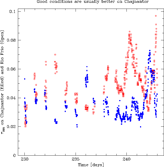
Figure: 2 Opacity time series for the two sites. Filled squares are
Chajnantor, open squares are Rio Frio, time is in days since 0 hours
UT, Jan 1, 1995. This plot only includes data when the radiometers at
both sites were functional.
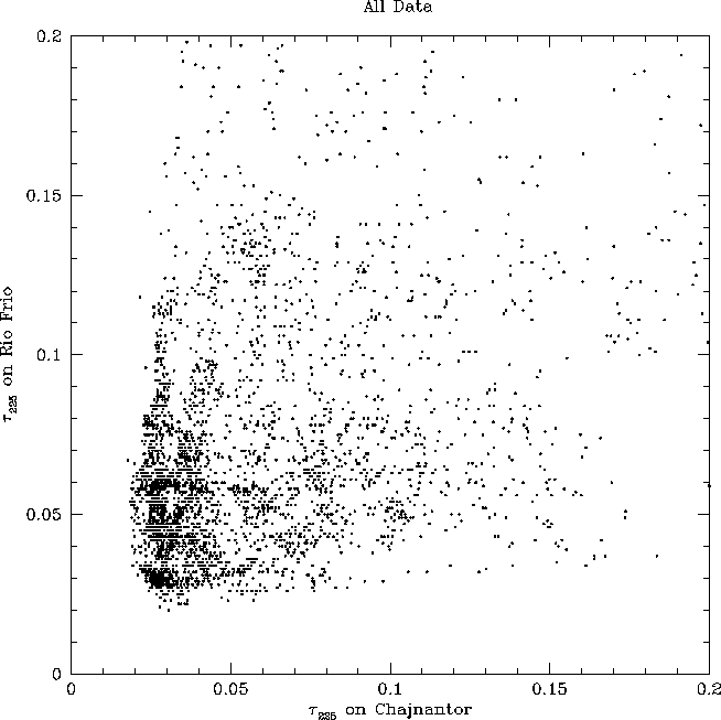
Figure: 3 Rio Frio opacity plotted against Chajnantor opacity. This plot only includes data when the radiometers
at both sites were functional.
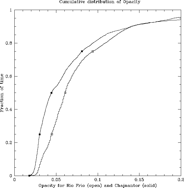
Figure: 4 Cumulative distributions and quartiles of the opacity at Rio Frio (open boxes)
and Chajnantor (filled boxes). This plot only includes data when the radiometers
at both sites were functional.
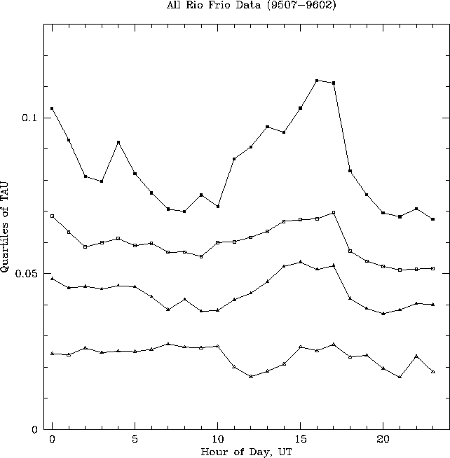
Figure: 5 Diurnal fluctuations of the opacity using all radiometer data from Rio Frio.
The variations are very small, and only during the worst conditions do day time
opacities show a marked increase over the night time values.
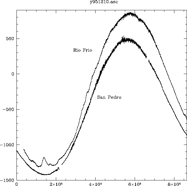
Figure: 6 The raw phase data from Rio Frio (bumpy line) and Chajnantor (line with
two small breaks) for one day indicates that there are some medium time scale
(10-60 minutes) phase excursions in the Rio Frio data. These phase excursions
do not appear to be correlated with any measured weather data.
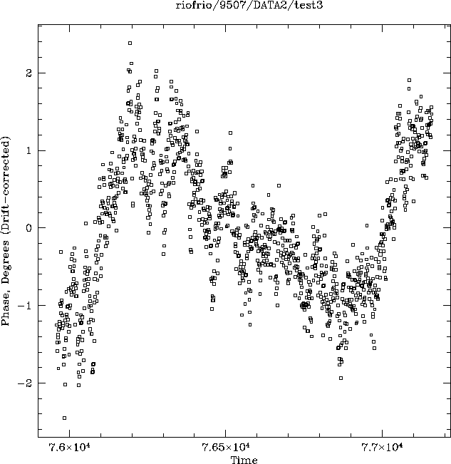
Figure: 7 We zoom in to take a close look at one of the anomalous phase excursions after
a quadratic trend has been removed from a 20 minute phase time series. The dominant ``z''
shape is probably instrumental rather than atmospheric, and will leave some residual effect
on 10 minute phase time series.
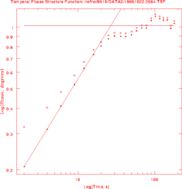
Figure: 8 The calculated temporal phase structure function at a time of good phase stability (open boxes)
and the structure function after removing the 0.25 degree noise term.
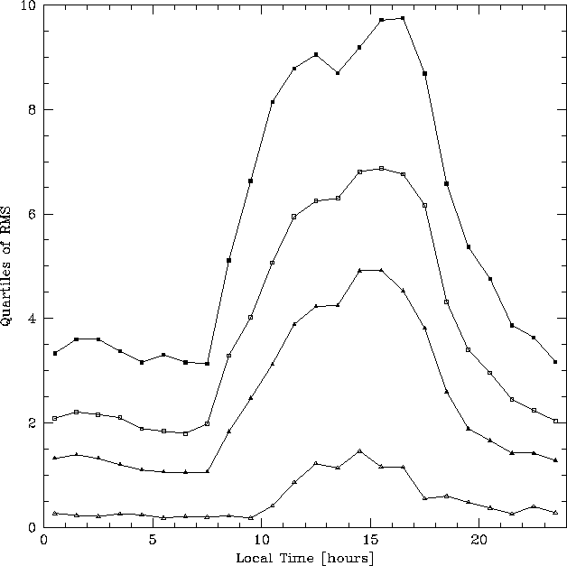
Figure: 9 Diurnal variations of the rms phase in degrees over 600 s using all Rio Frio phase stability data.
The lowest curve is for the best phase conditions observed, and the other three
curves are for the first, second, and third quartiles rms phases.
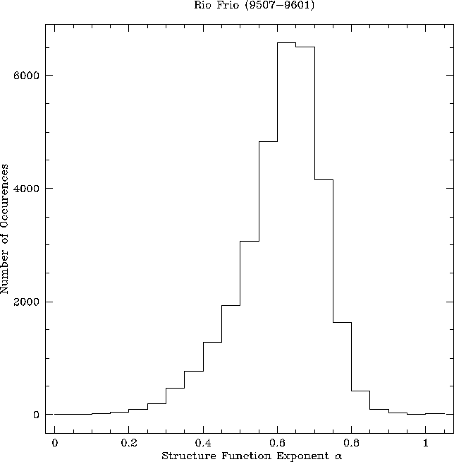
Figure: 10 Histogram of the phase structure function power law exponents sing all
phase data from the Rio Frio site. It is reassuring that nearly all exponents lie within
the 0.33 to 0.83 theoretical range.
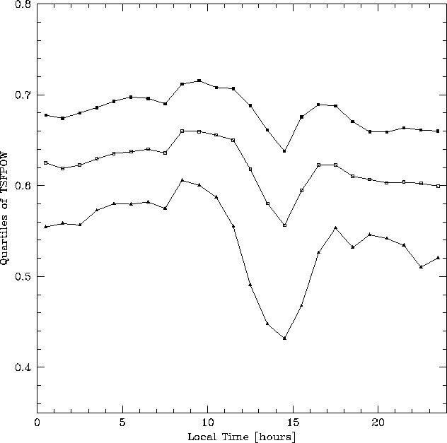
Figure: 11 Diurnal variations of the first, second, and third quartile values of the
structure function exponent from all phase data from the Rio Frio site.
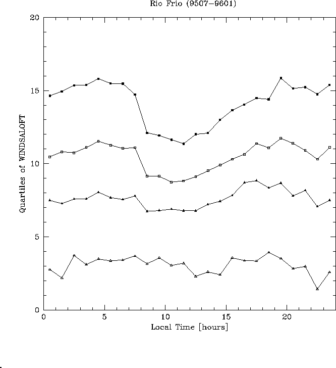
Figure: 12 Diurnal variations in the speed of the turbulent water vapor above the interferometer.
The lowest calculated speed of the ``wind aloft'' in m/s, followed by the first, second, and third quartile values
are shown for all phase data from the Rio Frio site.
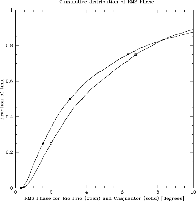
Figure: 13 Cumulative distribution of the rms phase at the Rio Frio and Chajnantor sites.
This plot only includes data when the radio seeing monitors at both sites were functional.
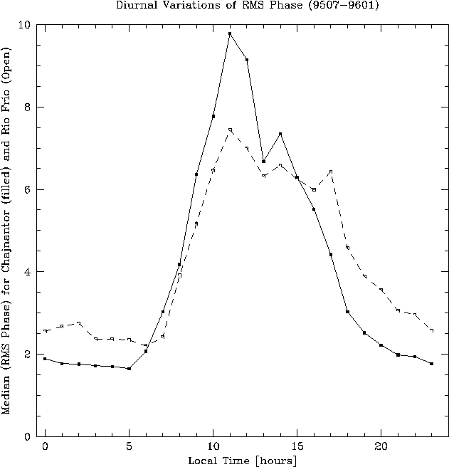
Figure: 14 Diurnal variation of the median rms phase on the Rio Frio
(solid lines, filled boxes) and Chajnantor (dashed lines, empty boxes)
sites. This plot only includes data when the radio seeing monitors at
both sites were functional.
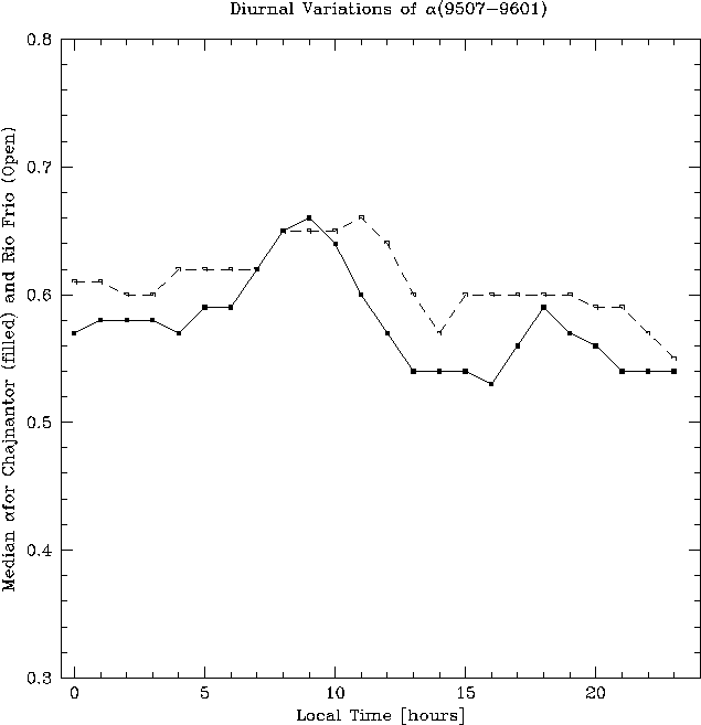
Figure: 15 Diurnal variation of the median structure function exponent
on the Rio Frio (solid lines, filled boxes) and Chajnantor (dashed
lines, empty boxes) sites. This plot only includes data when the
radio seeing monitors at both sites were functional.
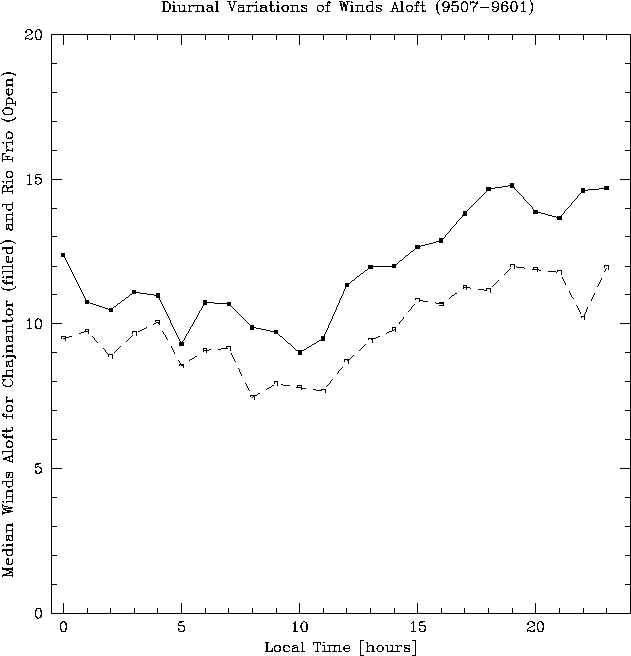
Figure: 16 Diurnal variation of the median speed of the turbulent water
vapor above the Rio Frio (solid lines, filled boxes) and Chajnantor
(dashed lines, empty boxes) sites. This plot only includes data when
the radio seeing monitors at both sites were functional.