Return to Memolist
MMA Memo 136: Correcting for Decorrelation Due to Atmospheric Phase Errors
M.A. Holdaway and F.N. Owen
National Radio Astronomy Observatory
Socorro, NM 87801
September 20, 1995
Abstract:
We explore how image reconstruction degrades with uncorrected phase
errors and how corrections can be made for the mean decorrelation even
when we cannot correct for the actual phase errors. Correcting the
visibility amplitude for the mean decorrelation as a function of
baseline length improves the reconstructed image. Deconvolving the
dirty image by a point spread function which includes the statistical
effects of the phase errors as well as the effects of the incomplete
Fourier plane sampling results in superior images. The latter
technique permits very good image reconstruction even in the presence
of phase errors as high as 70 degrees, and permits some sort of
reconstruction in the presence of 105 degree rms phase errors. The MMA's
phase error specifications need to be reevaluated in light of these
new imaging techniques.
Atmospheric phase errors cause trouble for millimeter interferometers:
systematic phase errors result in gross positional errors; systematic
and random phase errors limit the image quality; random phase errors
limit the sensitivity through decorrelation of the visibilities; time
dependent decorrelation results in flux scale errors; and since the
phase errors (and hence decorrelation) grow worse with baseline,
atmospheric phase errors limit the possible resolution of an array.
The best line of defense against this tropospheric menace is to avoid
the issue entirely by observing on a good site, on short baselines or
at low frequencies where the phase errors will be lower. Since the
science demands observations on long baselines and at high
frequencies, we are pushed to use an active phase calibration
technique which limits the residual phase errors to an acceptably low
level. We have written about a specification of 30 degree rms residual
phase error per baseline for any such exotic phase calibration
technique (Holdaway, 1992). We think the strongest justification for
this specification is the amplitude loss due to decorrelation given by
 (Thompson, Moran, and Swenson, 1986), where
  is the rms phase error per visibility in radians.
Hence, 30 degree rms phase errors will decrease the amplitude of the
visibilities by 0.87. If the time scale of the phase fluctuations is
larger than the integration time, the image flux will be down by 0.87,
and the phase fluctuations will scatter flux through the image.
However, this 13% loss in sensitivity is fairly modest, and we would
probably be willing to live with a higher loss in sensitivity if we
were performing exploratory observations at very high frequencies and
we could somehow correct for the effects of the decorrelation.
Hence, we should ask what level of phase errors will still permit
reasonable imaging, and can anything be done to correct for the image
errors caused by baseline dependent decorrelation?
is the rms phase error per visibility in radians.
Hence, 30 degree rms phase errors will decrease the amplitude of the
visibilities by 0.87. If the time scale of the phase fluctuations is
larger than the integration time, the image flux will be down by 0.87,
and the phase fluctuations will scatter flux through the image.
However, this 13% loss in sensitivity is fairly modest, and we would
probably be willing to live with a higher loss in sensitivity if we
were performing exploratory observations at very high frequencies and
we could somehow correct for the effects of the decorrelation.
Hence, we should ask what level of phase errors will still permit
reasonable imaging, and can anything be done to correct for the image
errors caused by baseline dependent decorrelation?
Holdaway (1992) investigated image quality as a function of phase error
magnitude for point sources and concluded that even with 30 degree rms
phase errors, reasonable imaging with dynamic range of about 200:1 was
still possible. In considering a more complex source, a more
realistic atmospheric model with baseline dependent phase errors
should be employed, as in the atmospheric simulations of Holdaway
(1991). The particular atmospheric phase screen model used in the
simulations described below results in phase errors which increase as
the baseline raised to the 0.33 power, which is seen during good
conditions on the potential MMA sites. During poorer conditions, the
phase errors usually increase more steeply with baseline length, at
least out to baselines of 300 m, but the basic conclusions derived
from this work should be independent of the details of the phase
structure function. Simulations were performed with a random circular
array of 1 km maximum baseline. Samples on the (u, v) tracks were
calculated for 5 s integrations, the standard M31 HII region model
image was Fourier transformed and degridded into the simulated
(u, v)
points. We assumed no decorrelation occurred on time scales less than
5 s. The entire simulated data set was 18 minutes long, or ten
atmospheric crossing times of the array's longest baseline. The
amplitude of the phase screen was scaled as required, the phase screen
was ``blown'' over the array with frozen turbulence at a velocity of
10 m/s, and the phase errors were then applied to the antennas below,
thereby corrupting the phase of the visibilities. No other errors
were added to the visibilities.
For the purpose of representing the typical level of phase fluctuations
graphically, we parameterize each of the scaled atmospheres in
the rms phase error calculated over the full 18 minute observation,
averaged over all baselines. Hence, a model atmosphere with mean
rms phase of 35 degrees will have some baselines with phase errors as
high as 50 degrees.
We have imaged the corrupted visibilities in three different ways:
- we have imaged the source without any decorrelation
correction, Fourier transforming the uniformly weighted
gridded visibilities and deconvolving using the maximum
entropy method (MEM) of Cornwell and Evans (1984).
- we have corrected the amplitudes of the target source visibilities
based on the decorrelation observed in the calibrator source,
followed by the Fourier transform and deconvolution.
- we have imaged the source by Fourier transforming the
uncorrected visibilities and then deconvolving with a beam
which includes both the effects of the sampling in the Foureir plane
and the statistical effects of the phase errors.
We expound on the two correction techniques below.
We have simulated calibrator observations which look through the same
model atmosphere as the target source, but removed by more than 10
degrees on the sky. The details of the atmospheric phase time series
detected by the calibrator are not applicable to the target source,
and the target source visibilities have not been corrected for these
phase errors. This is the typical state of current interferometer
observations: the calibration is not fast enough to track the
atmospheric phase errors. We average the calibrator visibilities to
determine the extent of the decorrelation. The statistics of the
phase errors on each baseline of the calibrator will be similar to the
statistics of the phase errors on the target source, and the level of
decorrelation will be comparable. Ignoring the phase of the averaged
calibrator data, we can make a table of baseline based amplitude
corrections given by

We then average the target source visibilities to the same extent,
increase the averaged target source visibilities' amplitudes by
 , Fourier transform and deconvolve by the standard Fourier
sampling based point spread function.
, Fourier transform and deconvolve by the standard Fourier
sampling based point spread function.
Averaging the visibilities in time will result in smaller phase
errors, but will also limit the field of view, so this method will
only work on smallish sources. The extent of the decorrelation and
the resulting images will depend upon the averaging time used. In
order to correct for the full  decorrelation, we must average the visibilities over several baseline
crossing times. The short baselines in our simulations are maximally
decorrelated after averaging for a minute, while the 1 km baselines
require averaging over the full 18 minute observation.
decorrelation, we must average the visibilities over several baseline
crossing times. The short baselines in our simulations are maximally
decorrelated after averaging for a minute, while the 1 km baselines
require averaging over the full 18 minute observation.
In radio astronomy, the Fourier transform of the sampled visibilities
with no phase errors yields the dirty image


where  is the visibility function and
  is the sampling
function. By the convolution theorem, multiplication by the sampling
function
is the sampling
function. By the convolution theorem, multiplication by the sampling
function  leads to a convolution of the true image by a point
spread function which is given by the Fourier transform of
leads to a convolution of the true image by a point
spread function which is given by the Fourier transform of  .
In the presence of antenna based phase errors
.
In the presence of antenna based phase errors  ,
,


where  represents the combined effects of the phases in the
Fourier plane. Hence, the dirty image will be the true image
convolved with a point spread function given by
represents the combined effects of the phases in the
Fourier plane. Hence, the dirty image will be the true image
convolved with a point spread function given by

The problem with this formalism is that we do not know  .
.
There is a nice analog to this approach in optical astronomical
imaging, in which the resolution is limited by phase fluctuations in
the atmosphere which are generally too fast to correct. A typical
optical field of view contains several bright stars, and the profiles
of these stars can be used to derive an effective point spread
function representing the statistical effects of the atmosphere. The
phase errors are occurring so quickly that we have thousands of
independent instantiations of the phase errors, and even though the
phase errors are not known in any detail, the form of T(u)can be
determined. Some degree of superresolution can then be achieved by
deconvolving the effects of this point spread function from the entire
image.
The situation at millimeter frequencies is different from the optical
situation in two respects: we will have tens of crossing times of the
turbulence over our aperture instead of thousands, and it will be rare
to encounter bright point sources in the field of interest (Holdaway,
Owen, and Rupen, 1994). Holdaway and Owen (1995) have recently
analized the residual phase errors which result from imperfect
atmospheric cancellation when switching between the target source and
a nearby calibrator. Phase fluctuations which occur faster than the
switching time scale cannot be corrected, and will result in
significant decorrelation if the residual phase errors are about
30 degrees or larger. However, it is possible to use the statistics of
the phase errors as measured on a calibrator to simulate an effective
point spread function which would include the effects of both the
incomplete Fourier sampling and the phase jitter. We can determine
the phase structure function from the calibrator phase time series,
which allows us to construct a model phase screen which will have the
same statistical properties as the actual atmosphere, but which will
not have the correct detailed phases. Hence, deconvolving with the
point spread function which includes phase errors from this model
atmosphere can correct for the decorrelation, as can the amplitude
correction scheme. As in the amplitude correction scheme, details of
the phase time series derived from the model atmosphere will be wrong,
so errors will be made. However, on average, the model phases will
affect the point spread function in a manner which is representative
of how the actual target source phase errors scatter flux in the
target source. We found that superior results were achieved when we
calculated the effective point spread function, including phase
errors, from several (ten) different model atmospheres, averaged the
different model point spread functions, and then deconvolved the dirty
image with this effective point spread function.
This method, or the statistical deconvolution of phase errors,
is quite similar to correcting the decorrelated amplitudes. After
averaging several effective PSF's, the phases will be small, so the
effective PSF will be dominated by the Fourier sampling and the
amplitude decorrelation. Consider the case of perfect Fourier
sampling, so the effective PSF is due entirely to the amplitude
decorrelation. Deconvolving by this function is equivalent to
dividing the Fourier transform of the image by the Fourier transform
of the effective PSF, or boosting up the amplitudes of the outer
visibilities as performed when correcting the decorrelated amplitudes.
In both the amplitude correction and the statistical deconvolution of
phase errors schemes, the results are dependent upon the post
observation averaging time in a complicated manner which has not yet
been fully explored.
We can compare the success of these various imaging pathways on a wide
range of simulated data through standard measures of imaging success
such as the dynamic range and fidelity index, or more subjectively
through looking at the final reconstructions side by side. The
fidelity image, first introduced by Cornwell, Holdaway, and Uson
(1993) to measure the success of image simulation, is an image of the
quantity one over the fractional pixel error. The fidelity index,
renamed here as the median fidelity, is the median pixel value
of the fidelity image after clipping the low fidelity points which
occur in very faint pixels and pixels whose fidelity is very high by
chance. Since most pixels in our model images are fairly low
brightness, the median fidelity emphasizes the great sea of low
brightness pixels. A reconstruction with a median fidelity of 20 is
considered highly successful. For the current investigation, we
further define the first moment of the fidelity, which is the mean
fidelity weighted by the pixel value raised to the first power. The
first moment fidelity is less sensitive to errors in the low
brightness pixels and better gauges the success of the reconstruction
of the bright, compact features in the image. Both fidelities measure
the quality of image reconstruction on source, while the dynamic
range measures the level of error off source relative to the
brightest reconstructed feature.
Figure 1 shows the images of a series of simulations
with  ,
,  ,
,  , and
, and  rms phase errors,
reconstructed with no correction, with the statistical phase
deconvolution, and with the the visibility amplitudes corrected. As
can be seen in the first column, as the phase errors increase, the
detailed structure of the source gets smeared and the flux scale goes
down. In the two correction techniques, the right flux scale is
maintained even in the presence of the largest phase errors. However,
inconsistencies in the amplitude corrected data scatter flux all over
the image, limiting the dynamic range as well as the fidelity of the
image. The statistical phase deconvolution method appears to be
superior and results in a very good reconstruction even with 70 degree
rms phase errors. Note that the point spread function used in the
statistical phase deconvolution method embodies both the loss in
resolution and the loss in sensitivity since the phase errors are
spreading the beam about and even cancelling part of the beam flux.
The resolution and sensitivity loss are represented as a function of
phase error in Figure 2. Finally, the dynamic range and
fidelities are plotted for each reconstruction scheme as a function of
rms phase error in Figure 3.
rms phase errors,
reconstructed with no correction, with the statistical phase
deconvolution, and with the the visibility amplitudes corrected. As
can be seen in the first column, as the phase errors increase, the
detailed structure of the source gets smeared and the flux scale goes
down. In the two correction techniques, the right flux scale is
maintained even in the presence of the largest phase errors. However,
inconsistencies in the amplitude corrected data scatter flux all over
the image, limiting the dynamic range as well as the fidelity of the
image. The statistical phase deconvolution method appears to be
superior and results in a very good reconstruction even with 70 degree
rms phase errors. Note that the point spread function used in the
statistical phase deconvolution method embodies both the loss in
resolution and the loss in sensitivity since the phase errors are
spreading the beam about and even cancelling part of the beam flux.
The resolution and sensitivity loss are represented as a function of
phase error in Figure 2. Finally, the dynamic range and
fidelities are plotted for each reconstruction scheme as a function of
rms phase error in Figure 3.
Under the assumption of baseline independent Gaussian residual phase
errors, such as might exist if Welch's total power monitor scheme or
Woody's water vapor spectrometer scheme were employed, a simpler
decorrelation correction might suffice. If the residual phase errors
were antenna dependent or time dependent, then one of the
decorrelation correction methods described here might improve the
imaging.
In the case of fast switching, the residual phase errors are
equal to the square root of the phase structure function
 for short baselines
  and saturate at
a value of
and saturate at
a value of  for baselines longer than
the effective switching length
for baselines longer than
the effective switching length  (Holdaway and Owen, 1995).
Since the decorrelation is baseline dependent under fast switching,
the decorrelation correction methods described above would be helpful.
(Holdaway and Owen, 1995).
Since the decorrelation is baseline dependent under fast switching,
the decorrelation correction methods described above would be helpful.
Currently, it is believed that reasonable imaging with the 40 element
mma should be possible with 30 degree rms phase errors, assuming the
phase errors do not maintain some systematic value over long times.
The 30 degree rms phase error per baselines specification comes from
point source simulations (dynamic range = 200:1; Holdaway, 1992) and
from sensitivity arguments (down to 0.87). These simulations show
that the MMA will be able to make high fidelity, moderate dynamic
range images of complex sources with rms phase errors of 70 degrees per
baseline (the worst baselines in this simulation actually had rms
phase errors of 100 degrees). The 70 degree phase errors will result in a
stiff penalty in sensitivity since the decorrelation is down to 0.47
on the typical baseline. A modest resolution loss of 17% also
occurs.
We propose that we have two levels of phase error specifications:
- The primary phase error specification of 30 degrees rms
per baseline will permit excellent imaging with almost
no loss in sensitivity from decorrelation. This should
be the primary goal of our phase correction schemes.
- The secondary phase error specification of 70 degrees rms
per baseline will still permit very good imaging with a loss
of 50% in sensitivity (a factor of four in time). This
secondary phase error specification reminds us that
atmospheric conditions which do not allow us to meet the
primary phase error specification are not lost.
This will be particularly important for an instrument
which is built on a suboptimal site and for observations
at very high frequencies.
In Table 4 we explore what the 30 degree and 70 degree phase error
specifications mean for observing on a 300 m baseline at Chajnantor in
Chile without any phase calibration. We list the phase
stability quartiles measured on the NRAO 300 m, 11.2 GHz site test
interferometer for the month of June 1995, and then determine what
frequency can be observed with 30 degree and 70 degree phase errors. Fast
switching can achieve an effective calibration baseline  of
about 50 m (Holdaway and Owen, 1995), and typical phase structure
function power law exponents are 0.7, so the post-calibration phase
errors would be
of
about 50 m (Holdaway and Owen, 1995), and typical phase structure
function power law exponents are 0.7, so the post-calibration phase
errors would be 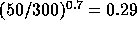 lower than the rms phase
errors measured on the 300 m baseline. These lower phase errors would
pertain to all baselines longer than 50 m, and would boost the peak
observing frequencies given in Table 4 by a factor of 3.5.
lower than the rms phase
errors measured on the 300 m baseline. These lower phase errors would
pertain to all baselines longer than 50 m, and would boost the peak
observing frequencies given in Table 4 by a factor of 3.5.
Special thanks to Claire Chandler who motivated this project, and may yet let her
name be on the auther list. Also, praise and thanks to Michael Rupen and Tim
Cornwell for nice but not yet implemented ideas. And thanks to Scott Foster
for technical support.
References
Cornwell, T.J., and Evans, 1984. A&A,
Cornwell, T.J., Holdaway, M.A., and Uson, J., 1993, A&A.
Holdaway, M.A, 1991, MMA Memo 68, ``A Millimeter Wavelength Phase
Stability Analysis of the South Baldy and Springerville Sites''.
Holdaway, M.A., 1992, MMA Memo 84, ``Possible Phase Calibration
Schemes for the MMA''.
Holdaway, M.A., Owen, F.N., and Rupen, M.P., 1994, MMA Memo 123,
``Source Counts at 90 GHz''.
Holdaway, M.A., and Owen, F.N., 1995, MMA Memo 126, ``A Test of Fast
Switching Phase Calibration with the VLA at 22 GHz''.
Holdaway, M.A., Radford, Simon J.E. , Owen, F.N., and Foster, Scott M.,
1995, MMA Memo 129, ``Data Processing for Site Test Interferometers''.
Thompson, A. Richard, Moran, James M., and Swenson, George W.,
Interferometry and Synthesis in Radio Astronomy, John Wiley & Sons,
New York, 1986.
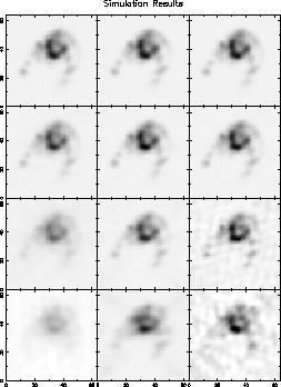
Figure 1: Three different reconstruction techniques (columns) applied to
four different magnitudes of phase errors (rows).
Column 1: imaging without any decorrelation correction.
Column 2: imaging with the statistical phase deconvolution.
Column 3: imaging with correction of the amplitudes only.
Row 1: 17 degree rms phase errors. Row 2: 35 degree rms phase errors.
Row 3: 70 degree rms phase errors. Row 4: 105 degree rms phase errors.
The statistical phase deconvolution technique is superior for
large phase errors.
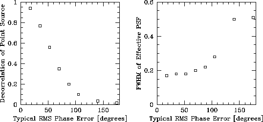
Figure 2: The phase errors will degrade the resolution as well as the
sensitivity. These figures illustrate how the resolution and
sensitivity at the highest resolution degrade with increasing phase
errors in our simulations. The sensitivity curve is consistent with  when we consider that the phase errors
at the highest resolution are higher than the mean phase errors we plot.
Also, the beam fitting is ill-conditioned in the high phase error case,
which explains why the resolution seems to flatten out at the right
side of the graph.
when we consider that the phase errors
at the highest resolution are higher than the mean phase errors we plot.
Also, the beam fitting is ill-conditioned in the high phase error case,
which explains why the resolution seems to flatten out at the right
side of the graph.

Figure 3: Three measures of image quality for the three imaging methods compared
in this memo: (a) Dynamic Range, defined as the image peak divided by the
off-source rms, (b) Median Fidelity, defined in the text, and (c)
First Moment Fidelity, defined in the text.
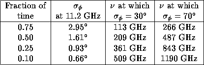
Table 1: How high a frequency could you operate the MMA in Chile
if 30 degree rms phase errors were required, and if 70 degree rms
phase errors were required? We present here the very conservative
estimates based on the NRAO 300 m, 11.2 GHz site test interferometer data
taken for the month of June 1995. The phase at 11.2 GHz was better than
2.95 degrees 75% of the time, indicating that 113 GHz observations would
have phase errors of less than 30 degrees more than 75% of the time, and
266 GHz observations would have phase errors of less than 70 degrees more
than 75% of the time. This table does not consider any form of calibration
aside from the decorrelation corrections described in this memo.
Active phase calibration could increase the maximum frequencies quoted in
this table by a factor of 3.5.