MMA Memo 129: Data Processing for Site Test Interferometers

M.A. Holdaway, Simon J.E. Radford, F.N. Owen, and Scott M. Foster
National Radio Astronomy Observatory

June 27, 1995

Abstract

The NRAO site test interferometers measure atmospheric path length fluctuations on a 300 m baseline. Here we describe data products derived from those measurements that can be used for site intercomparison and atmospheric modeling. As a demonstration of this analysis, we have processed two weeks of data from the instrument in Chile for 1995 May.

Introduction

To further evaluate possible sites for the MMA, NRAO has installed two site test interferometers, one at the VLBA site at 3720 m on Mauna Kea and the other at 5000 m near Cerro Chajnantor in northern Chile (near San Pedro de Atacama). These interferometers observe geostationary satellites to measure path length fluctuations due to inhomogeneously distributed water vapor. Unless they can be calibrated on short time scales, such fluctuations are a fundamental limit to the angular resolution of observations at millimeter and submillimeter wavelengths. From these measurements we wish to characterize the temporal and spatial variations of the path length, to estimate the natural seeing limits at given frequencies, and to estimate residual phase errors associated with a variety of phase calibration schemes. This information will ultimately be used to select the best site.

Interferometer and Phase Time Series

Each interferometer (Radford et al. 1995) has two 1.8 m antennas separated by 300 m. On Mauna Kea, the interferometer observes an unmodulated beacon at 11.7269 GHz on Gstar4 (105 W longitude, 29 elevation) and at Cerro Chajnantor, the instrument observes a 11.198 GHz beacon on Intelsat 601 (27.5 W longitude, 36 elevation). The power signal-to-noise ratio is 65 dB Hz on Mauna Kea and 58 dB Hz at Cerro Chajnantor. The received signals are amplified, downconverted, and transmitted to a central station, where they are further downconverted and the signal from one antenna is phase locked to the satellite beacon. These signals are then filtered, downconverted to 5 kHz, and digitized at 20 ksamples sec. The digital streams are multiplied and averaged for 1 s to extract the relative phase of the signals and the phase time series is written to a file in 60 s blocks along with engineering data. Graphical summaries of the data and of the instrument performance are faxed to our offices once or twice daily. The raw data are copied to tape and retrieved every month or two. Each block of sixty 1 s phases is perfectly synchronous, i. e., no samples are lost, and the gaps between the blocks are a few ms. This time series is the starting point for the analysis described here.

Desired Data Products

The primary data products that can be determined from 10 minute segments of the interferometer phase time series include:

The phase structure function (Tatarski, 1961) parameterized by the rms phase on the 300 m baseline, , and the exponent of a power law fit to the phase structure function, . The phase structure function , is given by
where is the distance between two antennas and is the atmospheric phase. Given the phase structure function, we can predict the rms phase on any baseline shorter than the measured baseline and extrapolate to the rms phase on longer baselines.
Any evidence for a change in the structure function exponent with baseline (time scale).
An estimate of the wind velocity at the mean height of the turbulent water vapor.

We can also construct some derived data products from these primary data products. These include:

The cumulative distributions of the rms phase measured on the 300 m baseline and predicted for a 100 m baseline using the structure function exponent. These are nice, intuitive plots that can easily be used to compare sites.
The three dimensional probability function
where is the rms phase on a reference baseline, is the exponent of the phase structure function power law (together and define the phase structure function), and v is the wind velocity aloft. This information is required to determine how well phase calibration techniques, such as fast switching or paired antenna phase calibration, will work.
The distribution of phase conditions with time of day or other parameters. This will be useful for planning the array use strategy.

Finally, the database of primary data products can be joined with the opacity database and the weather station database. The resulting joint database will provide many correlational data products that can be important diagnostics for understanding the dynamics of the atmosphere (Holdaway, Ishiguro, and Morita 1995).

Analysis of the phase time series and generation of the primary and derived data products require both new software and some experimentation. This memo documents our current view of the data processing used to obtain the primary data products. Analysis of correlations in the final joint database must wait until there is a substantial amount of site data from which we can draw statistical conclusions.

Data Calibration

An interferometer will detect atmospheric fluctuations on time scales ranging from 0 to a few times , where b is the physical baseline. Radiosonde measurements indicate typical winds aloft are 5 m s above Mauna Kea (Schwab 1992) and 10 m s above Cerro Chajnantor (Schwab private communication), so crossing times are 30 to 60 s. The phase structure function is the variance of the phase as a function of baseline, calculated over many atmospheric instantiations, usually approximated as many crossing times. The site test interferometer directly measures the phase structure function on a single 300 m baseline, and we require about 10 minutes of data to ensure many crossing times. Determining the baseline crossing time, which indicates the atmospheric velocity, also requires several crossing times.

On 10 minute time scales, however, there are significant phase variations caused by satellite motion and thermal changes in the instrument. These manifest themselves as gross, primarilly linear, trends in the data. When the satellite motion changes direction, or when temperature has a second time derivative, there can also be curvature in the instrumental contribution to the phase. Examination of the data indicates removal of a quadratic trend is sometimes required. If satellite motion causes five turns of phase per 24 hours, then the rms phase about the mean over 1024 s¹ would be inflated by as much as . Even after removing a linear trend from a 1024 s series, satellite motion could still contribute as much as to the rms phase, which is comparable to the expected atmospheric contribution during good conditions. In fact, some data indicate if a quadratic term were not removed, the rms phase over 1024 s would be inflated by as much as , much more than can be explained by the satellite motion. These data are probably affected by thermal drifts of the instrument. If a quadratic trend is fit over the 1024 s, however, satellite motion can contribute no more than to the rms phase, which is substantially less than the interferometer sensitivity or the best atmospheric conditions. Finally, subtracting a quadratic fit over a suitably long time will not alter the atmospheric phase fluctuations significantly. Simulations with typical power law exponents for the structure function indicate removing a quadratic trend from the 1024 s phase time series removes only about 1% of the atmospheric phase fluctuations.

In the presence of significant instrumental phase noise, the power spectrum of the interferometer phase is ill behaved at high frequencies. Hence, only those lower frequencies where the atmospheric phase fluctuations are much higher than the instrumental phase jitter can be used to estimate the phase structure function exponent. In addition, it is not at all straightforward to remove the instrumental power spectrum from the measured power spectrum. Holdaway, Ishiguro, and Morita (1995) demonstrate, however, the spatial phase structure function can be determined from the temporal structure function of the interferometer phase. Indeed this is sometimes better than using the power spectrum. For times shorter than the crossing time, the temporal structure function of the interferometer phase, , is related to the spatial structure function, , as

Furthermore, the temporal structure function is well behaved in the presence of instrumental noise. The temporal structure function of the instrumental phase can be removed from the temporal structure function of the measured phase by simple differencing,

In terms of the rms phase of the time series,

Simulations indicate that even after an instrumental term up to 5 times larger than the atmospheric phase fluctuations has been removed, the structure function exponent and the rms atmospheric phase can still be determined to an accuracy of about 20%. To demonstrate these concepts, Figure 1 shows the power spectrum of a phase time series from Chile that appears to be limited by white instrumental phase noise, and Figure 2 shows the temporal phase structure function of the same time series, both before and after the instrumental term has been subtracted.

During the best conditions on Mauna Kea, we have not seen any times when instrumental phase noise obviously contributes to the structure function (and hence to the rms phase). At the summit, the best phase conditions measured on a 100 m baseline are about 0.1 degree rms at elevation, uncorrected for airmass effects (Masson, 1993). This scales to 0.23 degrees rms for a 300 m baseline if the structure function exponent is 0.75, the median value. These data are consistent with the lowest rms phases we measure at the VLBA site. The structure function exponent, , does tend however toward low values during the best phase conditions. This implies either the phase is dominated by water vapor in a thin screen or that is artificially flattened by instrumental noise on short time scales. We are still looking for an instrumental term in the Mauna Kea data, but until we find clear evidence, we do not plan to subtract any instrumental term from the data.

During the very best conditions on the Chilean site, on the other hand, there is a clear indication of instrumental noise in the temporal structure function. During those conditions, the square root of the structure function on short time scales saturates at about . Furthermore, we can iteratively subtract white noise from the structure function until it no longer flattens out on the shortest times. While the convergence rate varies for different data, this process converges to a common white noise amplitude of rms. When we subtract this noise from the phase structure functions, we find the power law fit stays reasonable down to 1-2 seconds. There may still be residual instrumental phase noise in the structure function at the level of rms, but this is much lower than the best atmospheric conditions and does not affect the structure function exponent.

The rms white noise in the temporal structure function of the interferometer phase corresponds to white noise in the measured phase time series. Hence, we subtract in quadrature from the rms phases to obtain the final calibrated value.

Primary Data Products

RMS Phase. The single most useful piece of information is the rms phase calculated for a time long compared to the crossing time, after the gross trends and phase noise have been removed. The cumulative distribution of the calibrated rms phase at 11.2 GHz on a 300 m baseline for May 10-26 on the Chile site is shown in Figure 3. For easy comparison with the SMA archive of data for Mauna Kea, we have converted this to microns of path length on a 100 m baseline using the structure function exponents derived below (Figure 4). The satellite elevation is , or 1.7 airmasses. Holdaway and Ishiguro (1995) and Treuhaft and Lanyi (1987) indicate that for short baselines (i.e., 300 m), the phase errors scale with the square root of the airmass. Hence to estimate the zenith path length fluctuations, we divide the measured fluctuations by 1.3.

Phase Structure Function Exponent. As indicated above, the exponent of the power law fit to the temporal structure function of the interferometer phase should be equal to the power law exponent of the spatial phase structure function. It is crucial to subtract the instrumental phase noise from the temporal structure function before fitting the power law. Otherwise, the noise will inflate the rms phase on short times during good conditions and lower by 0.1-0.3. We estimate residual instrumental noise is less than rms, which will lower only about 0.01 under the best atmospheric conditions. To avoid the affects of the residual instrumental noise, we ignore the 1 s point in fitting the exponent. The temporal structure function of the interferometer phase will also turn over at times comparable to the crossing time, so we must also include an upper time limit when fitting the power law. This upper limit is determined iteratively (see below).

In Figure 5 we show the structure function exponent plotted against the rms phase, before and after subtracting the noise. Even after correcting for the instrumental noise, still decreases somewhat during the lowest rms phase conditions. While this could be caused by residual instrumental noise, our estimates of any residual instrumental effect are consistent with a true decrease of the structure function exponent. This is also seen at Nobeyama (Holdaway, Ishiguro, and Morita 1995), where the instrumental function is smaller and the atmospheric phase fluctuations are larger. Exponents intermediate between the Kolmogorov values of 0.83 for a thick atmosphere and 0.33 for a thin atmosphere can be obtained from a superposition of a thick and a thin layer. Hence during the very good conditions in Chile, most of the turbulent water vapor seems to be in a thin ( m) layer. This may be the boundary of the inversion layer that often forms 500-1000 m above that site. In the distribution of (Figure 6), note the sharp cutoff near 0.83 and the more gradual approach to 0.33. The distribution of and the relationship between and rms phase suggest there is an everpresent thin turbulent water vapor layer and a thick turbulent water vapor layer of variable strength that dominates the phase in all but the best conditions.

``Corner Time'' and Velocity Aloft. The corner time, , analogous to Masson's (1993) corner frequency, is the time scale where the phase structure function turns over. We determine it iteratively: we fit a power law to the temporal phase structure function between 2 and 15 s time scales and find the mean phase between 50 and 300 second time scales. Unlike the power spectrum, the temporal phase structure function is (approximately) flat at long times. The time where the two fits intersect determines the new upper limit for the power law fit to the short time scales and the new lower limit for the mean of the long time scales. This process usually converges in three iterations. The corner time can be related to the crossing time of the array, and hence to the velocity, by atmospheric simulations (i.e., similar to Holdaway, Ishiguro, and Morita 1995). Simulations of atmospheres with velocities of 5-20 m and structure function exponents of 0.37-0.73 indicate tthe scaling between and atmospheric velocity v depends upon the structure function exponent,

where b is the nonprojected baseline, and

The uncertainty is estimated from the scatter in the simulations. To demonstrate the derived wind velocity aloft is actually measuring something, we provide a time series of the derived wind aloft and compare it to the measured surface wind velocity (Figure 7). The scatter in the derived wind aloft indicates there are probably some systematic errors causing uncertainties of more than a factor of 2 (see the scatter around time = 21.2), but also there are times when the scatter in the derived velocity is as low as 30% (see time = 20.8). Since the velocity of the winds aloft is a strong function of altitude and the interferometer samples the velocity at all altitudes where turbulent water vapor exists, we do not expect an unambiguous result. We are still investigating other possible means of estimating the wind velocity aloft from the interferometer phase time series.

Software Development

The data calibration, reduction, and analysis has been prototyped using UNIX shell scripts, SM, and SDE (Cornwell, Briggs, and Holdaway, 1995). Rather than using this heterogeneous assortment of software for the production data reduction, we plan to add the analysis to the data acquisition software, which is written with LabView. We will then calculate the primary data products for each 1024 s period at the site. A table of these statistics will be small enough to be transmitted daily by telephone.

References

Cornwell, T.J., Briggs, D.S., and Holdaway, M.A., 1995, SDE Users Guide.

Holdaway, M.A., and Ishiguro, Masato, 1995, MMA Memo 127, ``Dependence of Tropospheric Path Length Fluctuations on Airmass.''

Holdaway, M.A., Ishiguro, Masato, and Morita, K.-I., 1995, MMA Memo ???, ``Analysis of the Spatial and Temporal Phase Fluctuations Above Nobeyama.''

Masson, C.R., 1994, ``Atmospheric Effects and Calibration'', in Astronomy with Millimeter and Submillimeter Wave Interferometry, eds. Ishiguro and Welch.

Radford, S.J.E., et al., 1995, in preparation.

Schwab, F., 1992, MMA Memo 75, ``Lower Tropospheric Wind Speeds.....''.

Tatarski, V.I., 1961, Wave Propagation in a Turbulent Medium, McGraw-Hill, New York.

Treuhaft, Lanyi 1987, ``The Effect of the dynamic wet troposphere on radio interferometric measurements,'' Radio Science, Vol 22, No 2, 251-265.

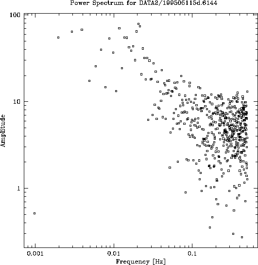
Figure 1: How instrumental phase noise affects the interferometer data: the square root of the power spectrum of a phase time series that is limited by white instrumental phase noise. The high frequencies are so corrupted by noise that a valid slope cannot be fit to the atmospheric fluctuations, and a turnover indicative of the atmospheric velocity is hard to discern. The power spectrum is also too poorly behaved to be able to remove an instrumental function.

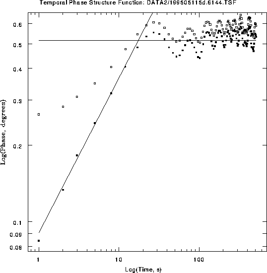
Figure 2: How instrumental phase noise affects the interferometer data: the square root of the temporal structure function of the same time series, both before the instrumental noise is removed (open squares) and after rms white noise is subtracted (filled squares). The sloping line is the fit to the atmospheric fluctuations and has a slope of . The intersection of the two lines defines the ``corner time'' . The oscillations on long times are probably an indication of the atmospheric velocity, but we have not yet exploited this information.

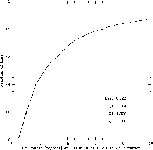
Figure: Cumulative distribution of rms phase in degrees at 11.2 GHz on a 300m baseline for 1995 May 10-26 on the Chile site. The satellite elevation is , so zenith fluctuations would be about 1.3 times lower.

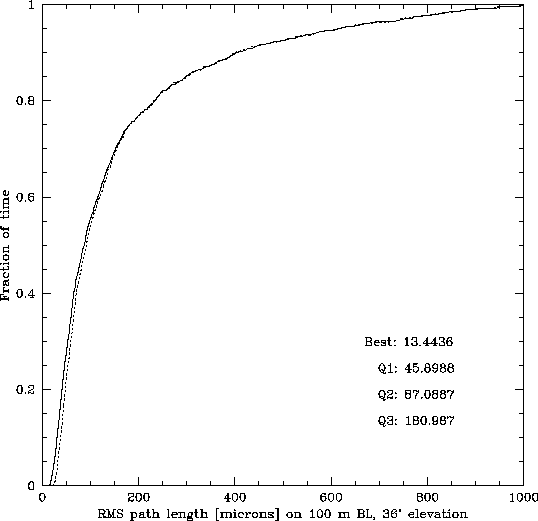
Figure 4: Cumulative distribution of rms path length in microns estimated for a 100m baseline for May 10-26 on the Chile site. The data have not been corrected to the zenith. The solid curve is the rms phase after the white noise has been subtracted, and the dashed curve is without calibration.

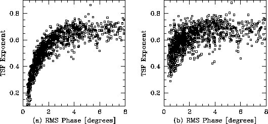
Figure 5: Structure function exponent plotted against the rms phase (a) prior to removing the instrumental term, and (b) after variance subtraction of a white noise. Data for 1995 May 10-26 on the Chile site.

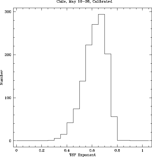
Figure 6: Distribution of the structure function exponent for 1995 May 10-26 on the Chile site.

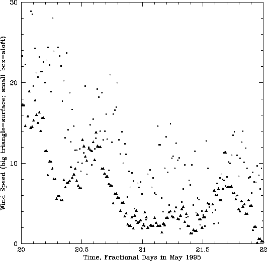
Figure 7: Derived velocity of the winds aloft as a function of time (small boxes) and measured surface wind velocity as a function of time (large triangles) for 1995 May 20-22 on the Chile site.

About this document ...

...s

Although powers of two have no special meaning for calculating the phase structure function, we have continued with a 1024 s time series in this memo as a vestage of using the power spectrum to determine the structure function exponent. Using the temporal structure function to determine the structure function exponent will allow a shorter time series, perhaps 600 s.